
Abstract
In this paper, we consider an inference problem about the drift parameter matrix of multivariate generalized Ornstein-Uhlenbeck processes with multiple unknown change-points in the case where the drift parameter matrix is suspected to satisfy some restrictions. The established results generalize in six ways some recent findings about univariate generalized Ornstein-Uhlenbeck processes. First, we consider a multivariate process with multiple change-points. Second, we weaken the assumptions underlying some recent findings and we derive the unrestricted estimator (UE) and the restricted estimator (RE). Third, we derive the asymptotic property of the UE and the RE. Fourth, we construct a test for testing the hypothesized constraint. Fifth, we establish the asymptotic power of the derived test and we prove that it is consistent. Sixth, we derive a class of shrinkage estimators (SEs) and its asymptotic distributional risk.


References
Chen, F. and Nkurunziza, S. (2016). A class of Stein-rules in multivariate regression model with structural changes. Scand. J. Statist. 43, 83–102.
Chen, F., Mamon, R. and Davison, M. (2017). Inference for a mean-reverting stochastic process with multiple change points. Electron. J. Statist. (EJS)11, 2199–2257.
Chen, F., Mamon, R. and Nkurunziza, S. (2018). Inference for a change-point problem under a generalised Ornstein-Uhlenbeck setting. Ann. Instit. Stat. Math. 70, 807–853.
Dehling, H., Franke, B. and Kott, T. (2010). Drift estimation for a periodic mean reversion process. Statist. Infer. Stoch. Process (SISP) 13, 175–192.
Dehling, H., Franke, B., Kott, T. and Kulperger, R. (2014). Change point testing for the drift parameters of a periodic mean reversion process. SISP17, 1–18.
Izenman, A.J. (2008). Modern Multivariate Statistical Techniques: Regression, Classification, and Manifold Learning. Springer Science & Business Media, LLC, New York.
Liptser, R.S. and Shiryaev, A.N. (2001). Statistics of Random Processes I:I. General Theory, 1. Springer, Berlin.
Nkurunziza, S. (2012). Shrinkage strategies in some multiple multi-factor dynamical systems. ESAIM: Probab. Statist. 16, 139–150.
Nkurunziza, S. (2013a). Extension of some important identities in shrinkage-pretest strategies. Metrika 76, 937–947.
Nkurunziza, S. (2013b). Preliminary test and estimation in some multifactor diffusion processes. Sankhyā: Indian J. Statist. Ser. A 75, 211–230.
Nkurunziza, S. and Ahmed, S. E. (2010). Shrinkage drift parameter estimation for multi-factor Ornstein-Uhlenbeck processes. Appl. Stoch. Models Bus. Ind.26, 103–124.
Nkurunziza, S. and Fu, K. (2019). Improved inference in generalized mean-reverting processes with multiple change-points. EJS 13, 1400–1442.
Nkurunziza, S. and Shen, L. (2020). Inference in a multivariate generalized mean-reverting process with a change-point. SISP 23, 199–226.
Nkurunziza, S. and Zhang, P.P. (2018). Estimation and testing in generalized mean-reverting processes with change-point. SISP 21, 191–215.
Perron, P. and Qu, Z. (2006). Estimating restricted structural change models. J. Econom. 134, 373–399.
Saleh, A.M.E. (2006). Theory of preliminary test and Stein-type estimation with applications 517. Wiley, New Jersey.
Sen, P.K. and Saleh, A.M.E. (1987). On preliminary test and shrinkage M-estimation in linear models. Ann. Statist. 15, 1580–1592.
Acknowledgement
The author would like to acknowledge the financial support received from the Natural Sciences and Engineering Research Council of Canada (NSERC). Further, the author would like to thank the referees for helpful comments ans useful insights.
Author information
Authors and Affiliations
Corresponding author
Additional information
Publisher’s Note
Springer Nature remains neutral with regard to jurisdictional claims in published maps and institutional affiliations.
Supported by Natural Sciences and Engineering Research Council of Canada
Appendices
Appendix A: Proofs of Some Fundamental Results
Proof 14 (Proof of Proposition 2.4).
We apply first the inequality \(\left \|\displaystyle {\sum \limits _{j=1}^{m+1}}b_{j}\right \|^{m_{0}}\leqslant (m+1)^{m_{0}-1}\displaystyle {\sum \limits _{j=1}^{m+1}}\|b_{j}\|^{m_{0}}\), for all \(b_{1}, b_{2}, \dots ,b_{m+1}\) d-column vectors. Thus, we have
\(\displaystyle \text {E}[\|\tilde {X}(t)\|^{m_{0}}]\leqslant 2^{m_{0}-1}(m+1)^{m_{0}-1}\sum \limits _{j=1}^{m+1}\text {E}[\|\tilde {h}_{j}(t)\|^{m_{0}} +\|\tilde {Z}_{j}(t)\|^{m_{0}}].\) Then,
Note that, \(\displaystyle \|\tilde {h}_{j}(t)\|^{m_{0}} =\displaystyle \Bigg \|e^{-A_{j}t}\sum \limits _{k=1}^{p}\mu _{k,j}{\int \limits }_{-\infty }^{t}e^{A_{j}s}\varphi _{k}(s)ds\Bigg \|^{m_{0}}.\) Then,
This gives, \(\displaystyle \sum \limits _{j=1}^{m+1}\|\tilde {h}_{j}(t)\|^{m_{0}}\!\leqslant \! p^{m_{0}-1}(m+1)^{m_{0}-1}K_{\mu }K_{\varphi }\displaystyle \sum \limits _{j=1}^{m+1}\left ({\int \limits }_{0}^{\infty }\|e^{-A_{j}s}\|ds\!\right )^{m_{0}}\) where Kμ and Kφ are strictly positive real numbers such that\(\displaystyle \sum \limits _{j=1}^{m+1} \sum \limits _{k=1}^{p}|\mu _{k,j}\) \(|^{m_{0}}\leqslant K_{\mu }\) and \(\|\varphi _{k}(s)\|\leqslant K_{\varphi }\) for all s, \(k=1,2,\dots ,m+1\). Then
\(\forall \ t\geqslant 0\). Further, we have
Then, by using Proposition 2.4 and Lemma 2.4, we get
and then,
Then, by combining Eqs. A.1, B.2 and A.3, we get
this completes the proof. □
Proof 15 (Proof of Proposition 2.5).
-
(i)
Recall that \(\displaystyle (C_{0}(\gamma _{m}))^{m_{0}}=\displaystyle \iota _{1}\sum \limits _{j=1}^{m+1} \left ({\int \limits }_{-\infty }^{0}\|e^{A_js}\|ds\right )^{m_{0}}+\iota _{2} \sum \limits _{j=1}^{m+1} \left \|{\int \limits }_{-\infty }^{0}\right .\) \(\left .e^{A_js}{\Sigma }^{1/2}d\tilde {W}_s\right \|^{m_{0}}+\iota _{3}\sum \limits _{j=1}^{m+1}\|X(\gamma _{j-1})\|^{m_{0}}\), with \(\iota _{1}=(3p(m+1))^{m_{0}-1}K^{*}\) \(d^{m_{0}/2}\), \(\iota _{2}=d^{m_{0}/2} (3(m+1))^{m_{0}-1}\) and \(\iota _{3}=(3(m+1))^{m_{0}-1}\). Then,
$$ \begin{array}{@{}rcl@{}} {{}}\text{E}\left( \displaystyle (C_{0}(\gamma_{m}))^{m_{0}}\right)&=&\displaystyle\iota_{1}\sum\limits_{j=1}^{m+1} \left[\left( {\int}_{-\infty}^{0}\|e^{A_{j}s}\|ds\right)^{m_{0}}\right]+\iota_{2} \sum\limits_{j=1}^{m+1} \text{E}\left[ \left\|{\int}_{-\infty}^{0}e^{A_{j}s}{\Sigma}^{1/2}d\tilde{W}_{s}\right\|^{m_{0}}\right]\\ &&+\iota_{3}\sum\limits_{j=1}^{m+1} \text{E}\left[\|X(\gamma_{j-1})\|^{m_{0}}\right] \end{array} $$and then, by combining Lemma 2.4 and Part (2) of Proposition 2.4, we have
$$ \begin{array}{@{}rcl@{}} &&{{}}\text{E}\left( \displaystyle (C_{0}(\gamma_{m}))^{m_{0}}\right)\leqslant\displaystyle\iota_{1}\sum\limits_{j=1}^{m+1} \left( {\int}_{-\infty}^{0}\|e^{A_{j}s}\|ds\right)^{m_{0}}+\iota_{2} \sum\limits_{j=1}^{m+1} \gamma_{2}(m_{0})\left[\text{trace}\left( (A_{j}+A^{\prime}_{j})^{-1}\right)\right]^{m_{0}/2}\\ &&{\kern30pt}+\iota_{3} \text{E}\left[\|X(0)\|^{m_{0}}\right] + \iota_{3}\sum\limits_{j=2}^{m+1}3^{(m_{0}-1)(j-1)}\text{E}\left( \|\mathbf{X}(0)\|^{m_{0}}\right) + d^{m_{0}/2}\\ &&{\kern30pt}\left( \max(2K_{2},c_{m_{0}}\|\mathbf{\Sigma}^{1/2}\|)\right)^{m_{0}}\times \sum\limits_{i=0}^{j-2}3^{(m_{0}-1)(i+1)}\\&& {\kern30pt}\left( \left( \lambda_{\max}\left( A_{j-1-i}^{-1}\right)\right)^{m_{0}} +(\lambda_{\max}(A_{j-1-i}^{-1}))^{m_{0}/2}\right). \end{array} $$Hence,
$$ \begin{array}{@{}rcl@{}} &&{{}}\text{E}\left( \displaystyle (C_{0}(\gamma_{m}))^{m_{0}}\right)\leqslant\displaystyle\iota_{1}\displaystyle\iota_{1}d^{m_{0}/2}2^{m_{0}}\sum\limits_{j=1}^{m+1} \left( \lambda_{\max}(A_{j}^{-1})\right)^{m_{0}}+\iota_{2} \sum\limits_{j=1}^{m+1} \gamma_{2}(m_{0})\left[\text{trace}\left( (A_{j}+A^{\prime}_{j})^{-1}\right)\right]^{m_{0}/2}\\ &&+\iota_{3} \text{E}\left[\|X(0)\|^{m_{0}}\right]+ \iota_{3}3^{m_{0}-1}\frac{3^{m(m_{0}-1)}-1}{3^{m_{0}-1}-1}\text{E}\left( \|\mathbf{X}(0)\|^{m_{0}}\right) \\&&+ d^{m_{0}/2} \left( \max(2K_{2},c_{m_{0}}\|\mathbf{\Sigma}^{1/2}\|)\right)^{m_{0}} \\ &&\times \sum\limits_{i=0}^{j-2}3^{(m_{0}-1)(i+1)}\left( \left( \lambda_{\max}\left( A_{j-1-i}^{-1}\right)\right)^{m_{0}} +(\lambda_{\max}(A_{j-1-i}^{-1}))^{m_{0}/2}\right)<\infty, \end{array} $$this proves Part (i).
-
(ii)
We recall first the inequality
$$ \begin{array}{@{}rcl@{}} \left\|\displaystyle{\sum\limits_{j=1}^{m+1}}b_{j}\right\|^{m_{0}}\leqslant (m+1)^{m_{0}-1}\displaystyle{\sum\limits_{j=1}^{m+1}}\|b_{j}\|^{m_{0}}, \end{array} $$(A.4)for all \(b_{1}, b_{2}, \dots ,b_{m+1}\) d-column vectors. From the inequality in Eq. A.4, we get
$$ \begin{array}{@{}rcl@{}} \|\tilde{\mathbf{X}}(t)-\mathbf{X}(t)\|^{m_{0}} \leqslant \ 3^{m_{0}-1}(m+1)^{m_{0}-1}\displaystyle{\sum\limits_{j=1}^{m+1}}\|\tilde{h}_{j}(t)-h_{j}(t)\|^{m_{0}}\\ +3^{m_{0}-1}(m+1)^{m_{0}-1}\displaystyle{\sum\limits_{j=1}^{m+1}}\|\tilde{Z}_{j}(t)-{Z}_{j}(t)\|^{m_{0}}\\ +3^{m_{0}-1}(m+1)^{m_{0}-1}\displaystyle{\sum\limits_{j=1}^{m+1}}\|e^{-A_{j}(t-\gamma_{j-1})}X(\gamma_{j-1})\|^{m_{0}}. \end{array} $$(A.5)Further, from Cauchy-Schwarz’s inequality, we have
$$ \begin{array}{@{}rcl@{}} &&\displaystyle\|\tilde{h}_{j}(t)-h_{j}(t)\|^{m_{0}} =\left\|e^{-A_{j}(t-\gamma_{j-1})}\sum\limits_{k=1}^{p}\mu_{k,j}{\int}_{-\infty}^{0}e^{A_{j}s}\varphi(s)ds\right\|^{m_{0}}\\ &\leqslant& \left\|e^{-A_{j}(t-\gamma_{j-1})}\right\|^{m_{0}}\left\|\sum\limits_{k=1}^{p}\mu_{k,j}{\int}_{-\infty}^{0}e^{A_{j}s}\varphi(s)ds\right\|^{m_{0}}, \end{array} $$then, by Jensen’s inequality,
$$ \begin{array}{@{}rcl@{}} &&\displaystyle\|\tilde{h}_{j}(t)-h_{j}(t)\|^{m_{0}}\leqslant p^{m_{0}-1}\|e^{-A_{j}(t-\gamma_{j-1})}\|^{m_{0}}\\ &&\times\sum\limits_{k=1}^{p}|\mu_{k,j}|^{m_{0}}\left( {\int}_{-\infty}^{0}\|e^{A_{j}s}\|ds\right)^{m_{0}-1}{\int}_{-\infty}^{0} \|e^{A_{j}s}\|\|\varphi(s)\|^{m_{0}}ds. \end{array} $$This gives,
$$ \begin{array}{@{}rcl@{}} {{}}\displaystyle\|\tilde{h}_{j}(t)-h_{j}(t)\|^{m_{0}} &\!\!\leqslant& p^{m_{0}-1}d^{m_{0}/2} K_{\mu} K_{\varphi}e^{-\lambda_{1}(A_{j})(t-\gamma_{j-1})/2}\left( {\int}_{-\infty}^{0}\|e^{A_{j}s}\|ds\right)^{m_{0}}, \end{array} $$(A.6)where Kμ > 0 and Kφ > 0 such that \(\|\mathbf {\varphi }(s)\|^{m_{0}}\!\leqslant \! K_{\varphi }\) and \(\displaystyle \sum \limits _{k=1}^{p}|\mu _{k,j}|^{m_{0}}\leqslant K_{\mu }\). Further, \(\displaystyle \|\tilde {Z}_j(t)-{Z}_{j}(t)\|^{m_{0}}=\left \| e^{-A_j(t-\gamma _{j-1})}{\int \limits }_{-\infty }^{0}e^{A_js}{\Sigma }^{1/2}d\tilde {W}_s\right \|^{m_{0}}\). Then,
$$ \begin{array}{@{}rcl@{}} {{}}\displaystyle\|\tilde{Z}_{j}(t)-{Z}_{j}(t)\|^{m_{0}}\leqslant d^{m_{0}/2} e^{-\lambda_{1}(A_{j})(t-\gamma_{j-1}) m_{0}/2}\left\|{\int}_{-\infty}^{0}e^{A_{j}s}{\Sigma}^{1/2}d\tilde{W}_{s}\right\|^{m_{0}}. \end{array} $$(A.7)$$ \begin{array}{@{}rcl@{}} {~}\sum\limits_{j=1}^{m+1}\displaystyle|\tilde{h}_{j}(t)-h_{j}(t)|^{m_{0}}\leqslant p^{m_{0}-1}d^{m_{0}/2} K^{*} \sum\limits_{j=1}^{m+1} e^{-\lambda_{1}(A_{j})m_{0}(t-\gamma_{j-1})/2}\left( {\int}_{-\infty}^{0}\|e^{A_{j}s}\|ds\right)^{m_{0}}, \\ \sum\limits_{j=1}^{m+1}\displaystyle|\tilde{Z}_{j}(t)-{Z}_{j}(t)|^{m_{0}}\leqslant d^{m_{0}/2}\sum\limits_{j=1}^{m+1} e^{-\lambda_{1}(A_{j})m_{0}(t-\gamma_{j-1})/2}\left\|{\int}_{-\infty}^{0}e^{A_{j}s}{\Sigma}^{1/2}d\tilde{W}_{s}\right\|^{m_{0}}, \end{array} $$\(t\geqslant \gamma _{m}\), with K∗ = KμKφ. Then,
$$ \begin{array}{@{}rcl@{}} {{}}\sum\limits_{j=1}^{m+1}\displaystyle|\tilde{h}_{j}(t)-h_{j}(t)|^{m_{0}}\leqslant p^{m_{0}-1}d^{m_{0}/2} K^{*} e^{-a_{(1)}m_{0}(t-\gamma_{m})/2}\sum\limits_{j=1}^{m+1} \left( {\int}_{-\infty}^{0}\|e^{A_{j}s}\|ds\right)^{m_{0}}, \\ \sum\limits_{j=1}^{m+1}\displaystyle|\tilde{Z}_{j}(t)-{Z}_{j}(t)|^{m_{0}}\leqslant d^{m_{0}/2} e^{-a_{(1)}m_{0}(t-\gamma_{m})/2}\sum\limits_{j=1}^{m+1} \left\|{\int}_{-\infty}^{0}e^{A_{j}s}{\Sigma}^{1/2}d\tilde{W}_{s}\right\|^{m_{0}}, \end{array} $$(A.8)\(t\geqslant \gamma _{m}\). Then, by Eqs. A.5 and A.8, we have
$$ \begin{array}{@{}rcl@{}} |\tilde{\mathbf{X}}(t)-\mathbf{X}(t)|^{m_{0}}\leqslant (C_{0}(\gamma_{m}))^{m_{0}}e^{-a_{(1)}m_{0}(t-\gamma_{m})/2}, \quad{ } t\geqslant\gamma_{m}, \end{array} $$(A.9)where
$$ \begin{array}{@{}rcl@{}} {{}}\displaystyle (C_{0}(\gamma_{m}))^{m_{0}} = \iota_{1}\sum\limits_{j=1}^{m+1} \left( {\int}_{-\infty}^{0}\|e^{A_{j}s}\|ds\right)^{m_{0}} + \iota_{2} \sum\limits_{j=1}^{m+1} \left\|{\int}_{-\infty}^{0}e^{A_{j}s}{\Sigma}^{1/2}d\tilde{W}_{s}\right\|^{m_{0}} + \iota_{3}\sum\limits_{j=1}^{m+1}\|X(\gamma_{j-1})\|^{m_{0}}, \end{array} $$with \(\iota _{1}=(3p(m+1))^{m_{0}-1}K^{*}d^{m_{0}/2}\), \(\iota _{2}=d^{m_{0}/2} (3(m+1))^{m_{0}-1}\) and \(\iota _{3}=(3(m+1))^{m_{0}-1}\). Then, the proof of Part (ii) follows from the fact that, from Part (i), \(\text {E}\left ((C_{0}(\gamma _{m}))^{m_{0}}\right )<\infty \).
-
(iii).
The convergence in \(L^{m_{0}}\) follows directly from Part (ii) together with the fact that the process \(\left \{\tilde {\mathbf {X}}(t)-\mathbf {X}(t):t\geqslant 0\right \}\) has continuous paths. Further, we from Part (ii), we have
$$ \begin{array}{@{}rcl@{}} {{}}\text{E}\left\{\displaystyle{\sup_{2^{n}\leqslant t\leqslant 2^{n+1}}}\big\|\tilde{\mathbf{X}}(t+\gamma_{m})-\mathbf{X}(t+\gamma_{m})\big\|^{m_{0}}\right\} \leqslant \text{E}\left( (C_{0}(\gamma_{m}))^{m_{0}}\right) e^{-a_{(1)}m_{0}2^{n}}, \end{array} $$and then
$$ \begin{array}{@{}rcl@{}} \displaystyle{\sum\limits_{n=1}^{\infty}}\text{E}\left\{\displaystyle{\sup_{2^{n}\leqslant t\leqslant 2^{n+1}}}\big\|\tilde{\mathbf{X}}(t+\gamma_{m})-\mathbf{X}(t+\gamma_{m})\big\|^{m_{0}}\right\}<\infty. \end{array} $$Therefore, together with the fact that \(\left \{\tilde {\mathbf {X}}(t)-\mathbf {X}(t):t\geqslant 0\right \}\) is a process with continuous paths, the convergence almost surely follows from Borel-Cantelli’s lemma.
-
(iv)
We have
$$ \begin{array}{@{}rcl@{}} &{}\big\|\tilde{\mathbf{X}}(t)\tilde{\mathbf{X}}^{\prime}(t)-\mathbf{X}(t)\mathbf{X}^{\prime}(t)\big\|^{m_{0}/2}= \big\|\tilde{\mathbf{X}}(t)\tilde{\mathbf{X}}^{\prime}(t)-\mathbf{X}(t)\tilde{\mathbf{X}}^{\prime}(t)+\mathbf{X}(t)\tilde{\mathbf{X}}^{\prime}(t)-\mathbf{X}(t)\mathbf{X}^{\prime}(t)\big\|^{m_{0}/2}\\ &{}\leqslant 2^{m_{0}/2-1}\|\tilde{\mathbf{X}}(t)-\mathbf{X}(t)\|^{m_{0}/2}\|\tilde{\mathbf{X}}(t)\|^{m_{0}/2}+ 2^{m_{0}/2-1}\|\tilde{\mathbf{X}}(t)-\mathbf{X}(t)\|^{m_{0}/2}\|\mathbf{X}(t)\|^{m_{0}/2}. \end{array} $$Then, together with Eq. A.9, for all \(t\geqslant \gamma _{m}\), we get
$$ \big\|\tilde{\mathbf{X}}(t)\tilde{\mathbf{X}}^{\prime}(t)-\mathbf{X}(t)\mathbf{X}^{\prime}(t)\big\|^{m_{0}/2}\leqslant (C_{0}(\gamma_{m}))^{m_{0}/2}e^{-a_{(1)}m_{0}(t-\gamma_{m})/2}\left( \|\tilde{\mathbf{X}}(t)\|^{m_{0}/2} + \|\mathbf{X}(t)\|^{m_{0}/2}\right). $$This gives
$$ \begin{array}{@{}rcl@{}} &&{{}}\sup_{2^{n}\leqslant t\leqslant 2^{n+1}}\big\|\tilde{\mathbf{X}}(t+\gamma_{m})\tilde{\mathbf{X}}^{\prime}(t+\gamma_{m})-\mathbf{X}(t+\gamma_{m})\mathbf{X}^{\prime}(t+\gamma_{m})\big\|^{m_{0}/2} \leqslant (C_{0}(\gamma_{m}))^{m_{0}/2} e^{-a_{(1)}m_{0}2^{n-1}} \\ &&{{}}\quad{ } \quad{ }\quad{ } \times\left( \sup_{2^{n}\leqslant t\leqslant 2^{n+1}}\|\tilde{\mathbf{X}}(t+\gamma_{m})\|^{m_{0}/2}+\sup_{2^{n}\leqslant t\leqslant 2^{n+1}}\|\mathbf{X}(t+\gamma_{m})\|^{m_{0}/2}\right). \end{array} $$(A.10)Then, since the processes \(\{\mathbf {X}(t):t\geqslant 0\}\) and \(\{\tilde {\mathbf {X}}(t):t\geqslant 0\}\) have continuous paths, we get
$$ \begin{array}{@{}rcl@{}} &&{{}}\sup_{2^{n}\leqslant t\leqslant 2^{n+1}}\big\|\tilde{\mathbf{X}}(t+\gamma_{m})\tilde{\mathbf{X}}^{\prime}(t+\gamma_{m})-\mathbf{X}(t+\gamma_{m})\mathbf{X}^{\prime}(t+\gamma_{m})\big\|^{m_{0}/2} \leqslant (C_{0}(\gamma_{m}))^{m_{0}/2} e^{-a_{(1)}m_{0}2^{n-1}}\\ &&\times \left( \|\tilde{\mathbf{X}}(t_{n}+\gamma_{m})\|^{m_{0}/2}+\|\mathbf{X}(t_{n}^{*}+\gamma_{m})\|^{m_{0}/2}\right), \quad{ } \end{array} $$(A.11)\( 2^{n}\leqslant t_{n},t_{n}^{*}\leqslant 2^{n+1}\). Further, by Cauchy-Schwarz’s inequality, we have
$$ \begin{array}{@{}rcl@{}} &&{{}}\text{E}\left[(C_{0}(\gamma_{m}))^{m_{0}/2}(\|\tilde{\mathbf{X}}(t_{n}+\gamma_{m})\|^{m_{0}/2}+\|\mathbf{X}(t_{n}^{*}+\gamma_{m})\|^{m_{0}/2})\right] \leqslant\left[\text{E}\left( (C_{0}(\gamma_{m}))^{m_{0}}\right)\right]^{1/2}\\ &&{}\quad{ } \quad{ } \quad{ } \quad{ } \quad{ } \quad{ } \quad{ } \quad{ } \quad{ } \times \left\{\text{E}\left[(\|\tilde{\mathbf{X}}(t_{n}+\gamma_{m})\|^{m_{0}/2}+\|\mathbf{X}(t_{n}^{*}+\gamma_{m})\|^{m_{0}/2})^{2}\right]\right\}^{1/2}\\ && {{}}\quad{ } \leqslant2^{1/2}\left[\text{E}\left( (C_{0}(\gamma_{m}))^{m_{0}}\right)\right]^{1/2} \left\{\text{E}\left[\|\tilde{\mathbf{X}}(t_{n}+\gamma_{m})\|^{m_{0}}\right]+\text{E}\left[\|\mathbf{X}(t_{n}^{*}+\gamma_{m})\|^{m_{0}}\right]\right\}^{1/2}. \end{array} $$As established in the proof of Part (i), \(\text {E}\left ((C_{0}(\gamma _{m}))^{m_{0}}\right )<\infty \). Further, from Propositions 2.4 and 2.4, \(\displaystyle \sup \limits _{t\geqslant 0} \text {E}[\|\mathbf {X}(t)\|^{m_{0}}]<\infty \) and \(\displaystyle \sup \limits _{t\geqslant 0} \text {E}[\|\tilde {\mathbf {X}}\) \((t)\|^{m_{0}}]<\infty \) and then, there exists K2 > 0 such that
$$ \begin{array}{@{}rcl@{}} &&{{}}\text{E}\left[(C_{0}(\gamma_{m}))^{m_{0}/2}(\|\tilde{\mathbf{X}}(t_{n}+\gamma_{m})\|^{m_{0}/2}+\|\mathbf{X}(t_{n}^{*}+\gamma_{m})\|^{m_{0}/2})\right] \leqslant 2^{1/2}\left[\text{E}\left( (C_{0}(\gamma_{m}))^{m_{0}}\right)\right]^{1/2}\\ &&{\kern98pt}\times\sup\limits_{t\geqslant 0}\{\left( \text{E}[\|\mathbf{X}(t)\|^{m_{0}}]+\text{E}[\|\tilde{\mathbf{X}}(t)\|^{m_{0}}]\right)^{\frac{1}{2}}\}\leqslant K_{2}<\infty. \end{array} $$Then
$$ \begin{array}{@{}rcl@{}} &&{{}}\text{E}\left\{\displaystyle{\sup_{2^{n}\leqslant t\leqslant 2^{n+1}}}\big\|\tilde{\mathbf{X}}(t+\gamma_{m})\tilde{\mathbf{X}}^{\prime}(t+\gamma_{m})\!-!\mathbf{X}(t+\gamma_{m})\mathbf{X}^{\prime}(t+\gamma_{m})\big\|^{m_{0}/2}\right\} \!\leqslant\! K_{0}^{*} K_{2}^{*} e^{-a_{(1)}m_{0}2^{n-1}}, \end{array} $$for some \(K_{0}^{*}>0\), \(K_{2}^{*}>0\), and then
$$ \begin{array}{@{}rcl@{}} &&{{}}\displaystyle{\sum\limits_{n=1}^{\infty}}\text{E}\left\{\displaystyle{\sup_{2^{n}\leqslant t\leqslant 2^{n+1}}}\big\|\tilde{\mathbf{X}}(t+\gamma_{m})\tilde{\mathbf{X}}^{\prime}(t+\gamma_{m})-\mathbf{X}(t+\gamma_{m})\mathbf{X}^{\prime}(t+\gamma_{m})\big\|^{m_{0}/2}\right\}<\infty. \end{array} $$Therefore, together with the fact that \(\left \{\tilde {\mathbf {X}}(t)\tilde {\mathbf {X}}^{\prime }(t)-\mathbf {X}(t)\mathbf {X}^{\prime }(t):t\geqslant 0\right \}\) is a process with continuous paths, Part (iv) follows from Borel-Cantelli’s lemma.
-
(v)
For \(0\leqslant a<b\leqslant 1\), by using the triangle inequality along with Cauchy-Schwarz and Jensen’s inequalities, we have
$$ \begin{array}{@{}rcl@{}} &&\left\|{\int}_{aT}^{bT}\tilde{\mathbf{X}}(t)\varphi^{\prime}(t)dt-{\int}_{aT}^{bT}\mathbf{X}(t)\varphi^{\prime}(t)dt\right\|^{m_{0}} \\&\leqslant& K_{\varphi}((b-a)T)^{m_{0}-1} {\int}_{aT}^{bT}\|\tilde{\mathbf{X}}(t)-\mathbf{X}(t)\|^{m_{0}}dt. \end{array} $$(A.12)Then, since 0 < (b − a)m− 1 < 1 for all \(0\leqslant a<b\leqslant 1\), we have
$$ \begin{array}{@{}rcl@{}} &&\sup_{0\leqslant a<b\leqslant 1}\left\|\frac{1}{T}{\int}_{aT}^{bT}\tilde{\mathbf{X}}(t)\varphi^{\prime}(t)dt-\frac{1}{T}{\int}_{aT}^{bT}\mathbf{X}(t)\varphi^{\prime}(t)dt\right\|^{m_{0}}\\ &\leqslant& \frac{K_{\varphi}}{T} {{\int}_{0}^{T}}\|\tilde{\mathbf{X}}(t)-\mathbf{X}(t)\|^{m_{0}}dt, \end{array} $$(A.13)and then, by using Part (iii) along with the continuous version of Kronecker’s lemma,
then, by combining this last relation with Eq. A.13, we get
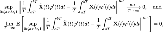
and then,
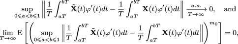
this proves the statement in Part (v).
-
(vi)
For \(0\leqslant a<b\leqslant 1\), by the triangle inequality, we have
$$ \begin{array}{@{}rcl@{}} \left\|\frac{1}{T}{\int}_{aT}^{bT}\tilde{\mathbf{X}}(t)\tilde{\mathbf{X}}^{\prime}(t)dt-\frac{1}{T}{\int}_{aT}^{bT}\mathbf{X}(t)\mathbf{X}^{\prime}(t)dt\right\|^{m_{0}/2}\\ \leqslant \frac{1}{T^{m_{0}/2}}\left( {\int}_{aT}^{bT}\|\tilde{\mathbf{X}}(t)\tilde{\mathbf{X}}^{\prime}(t)-\mathbf{X}(t)\mathbf{X}^{\prime}(t)\|dt\right)^{m_{0}/2}. \end{array} $$Then, by Jensen’s inequality, we have
$$ \begin{array}{@{}rcl@{}} \left\|\frac{1}{T}{\int}_{aT}^{bT}\tilde{\mathbf{X}}(t)\tilde{\mathbf{X}}^{\prime}(t)dt-\frac{1}{T}{\int}_{aT}^{bT}\mathbf{X}(t)\mathbf{X}^{\prime}(t)dt\right\|^{m_{0}/2}\\ \leqslant \frac{1}{T}(b-a)^{m_{0}/2-1}{\int}_{aT}^{bT}\|\tilde{\mathbf{X}}(t)\tilde{\mathbf{X}}^{\prime}(t)-\mathbf{X}(t)\mathbf{X}^{\prime}(t)\|^{m_{0}/2}dt, \end{array} $$then, since \(0< (b-a)^{m_{0}/2-1}<1\) for all \(0\leqslant a<b\leqslant 1\) whenever \(m_{0}\geqslant 2\), we get
$$ \begin{array}{@{}rcl@{}} &&\displaystyle \sup_{0\leqslant a<b\leqslant 1}\left( \Bigg\|\frac{1}{T}{\int}_{aT}^{bT}\tilde{\mathbf{X}}(t)\tilde{\mathbf{X}}^{\prime}(t)dt-\frac{1}{T}{\int}_{aT}^{bT}\mathbf{X}(t)\mathbf{X}^{\prime}(t)dt\Bigg\|^{m_{0}/2}\right)\\ &&{}\leqslant \frac{1}{T}{{\int}_{0}^{T}}\|\tilde{\mathbf{X}}(t)\tilde{\mathbf{X}}^{\prime}(t)-\mathbf{X}(t)\mathbf{X}^{\prime}(t)\|^{m_{0}/2}dt. \end{array} $$(A.14)Therefore, from Part (iv) along with the continuous version of Kronecker’s lemma, we get
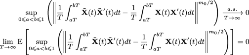
and then,
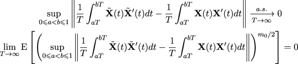
this completes the proof.


□
Proof 16 (Proof of Lemma 4.1).
-
(1).
Let \(\mathcal {C}_{T}(a, b)=\frac {1}{T}\displaystyle {{\int \limits }_{0}^{a T}}Y(t)dt-\frac {1}{T}\displaystyle {{\int \limits }_{0}^{b T}}Y(t)dt\). We have
$$ \begin{array}{@{}rcl@{}} \left\|\frac{1}{T}\displaystyle{{\int}_{\hat{a}T}^{\hat{b} T}}Y(t)dt-\frac{1}{T}\displaystyle{{\int}_{a T}^{b T}}Y(t)dt\right\| \leqslant \|\mathcal{C}_{T}(\hat{b}, b)\|+\|\mathcal{C}_{T}(\hat{a}, a)\|. \end{array} $$(A.15)It suffices to prove that \(\displaystyle \lim _{T\rightarrow \infty }\text {E}\left (\|\mathcal {C}_{T}(\hat {b}, b)\|\right )=0\). Let 𝜖 > 0, we have
$$ \begin{array}{@{}rcl@{}} \lim_{T\rightarrow\infty}P\left( |\hat{b}-b|\geqslant \epsilon\right)=0. \end{array} $$(A.16)Further, one can verify that
$$ \begin{array}{@{}rcl@{}} \|\mathcal{C}_{T}(\hat{b}, b)\|\leqslant \mathcal{I}_{11}(T)+\mathcal{I}_{12}(T)+\mathcal{I}_{21}(T)+\mathcal{I}_{22}(T) \end{array} $$(A.17)where
$$ \begin{array}{@{}rcl@{}} &&{{}}\mathcal{I}_{11}(T)=\frac{1}{T}\displaystyle{{\int}_{bT}^{\hat{b} T}}\|Y(t)\|dt \mathbb{I}_{\{b<\hat{b}\}}\mathbb{I}_{\left\{|\hat{b}-b|\geqslant \epsilon\right\}}, \mathcal{I}_{12}(T)=\frac{1}{T}\displaystyle{{\int}_{bT}^{\hat{b} T}}\|Y(t)\|dt \mathbb{I}_{\{b<\hat{b}\}}\mathbb{I}_{\left\{|\hat{b}-b|< \epsilon\right\}}\\ &&{{}}\mathcal{I}_{21}(T)=\frac{1}{T}\displaystyle{{\int}_{bT}^{\hat{b} T}}\|Y(t)\|dt \mathbb{I}_{\{b\geqslant \hat{b}\}}\mathbb{I}_{\left\{|\hat{b}-b|\geqslant \epsilon\right\}}, \mathcal{I}_{22}(T)=\frac{1}{T}\displaystyle{{\int}_{bT}^{\hat{b} T}}\|Y(t)\|dt \mathbb{I}_{\{b\geqslant \hat{b}\}}\mathbb{I}_{\left\{|\hat{b}-b|< \epsilon\right\}}. \end{array} $$We have
$$ \begin{array}{@{}rcl@{}} \text{ E}\left( \mathcal{I}_{11}(T)\right)\leqslant\frac{1}{T}\displaystyle{{\int}_{b T}^{T}}\text{E}\left[\|Y(t)\|\mathbb{I}_{\{bT<t<\hat{b}T\}}\mathbb{I}_{\{b<\hat{b}\}}\mathbb{I}_{\left\{\hat{b}\geqslant b+\epsilon\right\}}\right]dt. \end{array} $$(A.18)Then, by Hölder’s inequality
$$ \begin{array}{@{}rcl@{}} &&\text{ E}\left( \mathcal{I}_{11}(T)\right)\leqslant\frac{1}{T}\displaystyle{{\int}_{b T}^{T}}\left[\text{E}\left( \|Y(t)\|^{p}\right)\right]^{1/p} \left[\text{E}\left( \mathbb{I}_{\{bT<t<\hat{b}T\}}\mathbb{I}_{\{b<\hat{b}\}}\mathbb{I}_{\left\{\hat{b}\geqslant b+\epsilon\right\}}\right)\right]^{1/q}dt\\ &&{}\leqslant \frac{1}{T}\left[\displaystyle{{\int}_{b T}^{T}}\text{E}\left( \|Y(t)\|^{p}\right)dt\right]^{1/p} \left[\displaystyle{{\int}_{b T}^{ T}}\text{E}\left( \mathbb{I}_{\{bT<t<\hat{b}T\}}\mathbb{I}_{\{b<\hat{b}\}}\mathbb{I}_{\left\{\hat{b}\geqslant b+\epsilon\right\}}\right)dt\right]^{1/q} \end{array} $$with 1/q = 1 − 1/p, and since \(\left \{Y(t):t\geqslant 0\right \}\) is Lp-bounded, there exists K0 > 0 such that
$$ \begin{array}{@{}rcl@{}} \text{ E}\left( \mathcal{I}_{11}(T)\right)&\leqslant&\frac{K_{0}^{1/p}(1-b)^{1/p}T^{1/p}}{T}\left\{\text{E}\left[\displaystyle{{\int}_{b T}^{T}} \mathbb{I}_{\{bT<t<\hat{b}T\}}\mathbb{I}_{\{b<\hat{b}\}}\mathbb{I}_{\left\{\hat{b}\geqslant b+\epsilon\right\}}dt\right]\right\}^{1/q}\\ & & \leqslant\frac{K_{0}^{1/p}(1-b)^{1/p}T^{1/p}}{T}T^{1/q} \left[\text{E}\left( |\hat{b}-b|\right)\right]^{1/q} \end{array} $$this gives
$$ \begin{array}{@{}rcl@{}} \text{ E}\left( \mathcal{I}_{11}(T)\right)\leqslant K_{0}^{1/p}(1-b)^{1/p}\left[\text{E}\left( |\hat{b}-b|\right)\right]^{1/q}, \end{array} $$(A.19)and then, by combining Eqs. A.16 and A.19 along with Lebesgue dominated convergence theorem, we get \(\displaystyle {\lim _{T\rightarrow \infty }}\text { E}\left (\mathcal {I}_{11}(T)\right )=0\). Further, we have
$$ \begin{array}{@{}rcl@{}} \text{E}\left( \mathcal{I}_{12}(T)\right)\leqslant \frac{1}{T}\displaystyle{{\int}_{b T}^{bT+\epsilon T}}\text{E}\left[\|Y(t)\|\mathbb{I}_{\{bT<t<\hat{b}T\}}\mathbb{I}_{\{b<\hat{b}\}}\mathbb{I}_{\left\{b<\hat{b}< b+\epsilon\right\}}\right]dt. \end{array} $$Then, by Hölder’s inequality
$$ \begin{array}{@{}rcl@{}} &&{}\text{ E}\left( \mathcal{I}_{12}(T)\right)\leqslant\frac{1}{T}\displaystyle{{\int}_{b T}^{bT+\epsilon T}}\left[\text{E}\left( \|Y(t)\|^{p}\right)\right]^{1/p} \left[\text{E}\left( \mathbb{I}_{\{bT<t<\hat{b}T\}}\mathbb{I}_{\{b<\hat{b}\}}\mathbb{I}_{\left\{b<\hat{b}< b+\epsilon\right\}}\right)\right]^{1/q}dt\\ &&{}\leqslant \frac{1}{T}\left[\displaystyle{{\int}_{b T}^{bT+\epsilon T}}\text{E}\left( \|Y(t)\|^{p}\right)dt\right]^{1/p} \left[\displaystyle{{\int}_{b T}^{bT+\epsilon T}}\text{E}\left( \mathbb{I}_{\{bT<t<\hat{b}T\}}\mathbb{I}_{\{b<\hat{b}\}}\mathbb{I}_{\left\{b<\hat{b}< b+\epsilon\right\}}\right)dt\right]^{1/q} \end{array} $$with 1/q = 1 − 1/p, and since \(\left \{Y(t):t\geqslant 0\right \}\) is Lp-bounded, there exists K0 > 0 such that
$$ \begin{array}{@{}rcl@{}} {}\text{E}\left( \mathcal{I}_{12}(T)\right)&&\!\!\!\!\leqslant\frac{K_{0}^{1/p}\epsilon^{1/p}T^{1/p}}{T}\left\{\text{\!E\!}\left[\displaystyle{{\int}_{b T}^{bT+\epsilon T}} \mathbb{I}_{\{bT<t<\hat{b}T\}}\mathbb{I}_{\{b<\hat{b}\}}\mathbb{I}_{\left\{b<\hat{b}< b+\epsilon\right\}}dt\right]\right\}^{1/q}\\ &&\!\!\!\leqslant\frac{K_{0}^{1/p}\epsilon^{1/p}T^{1/p}}{T}T^{1/q} \left[\text{E}\left( |\hat{b}-b|\mathbb{I}_{\left\{|\hat{b}-b|<\epsilon\right\}}\right)\right]^{1/q}<K_{0}^{1/p}\epsilon, \end{array} $$this proves that \(\displaystyle {\lim _{T\rightarrow \infty }}\text { E}\left (\mathcal {I}_{12}(T)\right )=0\). By using the similar techniques, one can prove that \(\displaystyle {\lim _{T\rightarrow \infty }}\text { E}\left (\mathcal {I}_{21}(T)\right )=\displaystyle {\lim _{T\rightarrow \infty }}\text { E}\left (\mathcal {I}_{22}(T)\right )=0\), this proves the first statement.
-
(2).
Obviously,
 (A.20)
Further, we have
$$ \begin{array}{@{}rcl@{}} &&{}\text{E}\left( \mathcal{I}^{p}_{12}(T)\right)\leqslant \frac{1}{T^{p}}\text{E}\left\{\left[\displaystyle{{\int}_{b T}^{bT+\epsilon T}}\left( \displaystyle{\sup_{bT\leqslant t \leqslant bT+\epsilon T}}(\|Y(t)\|)\right)\mathbb{I}_{\{bT<t<\hat{b}T\}}\mathbb{I}_{\{b<\hat{b}\}}\mathbb{I}_{\left\{b<\hat{b}< b+\epsilon\right\}}dt\right]^{p}\right\}\\ &&\leqslant \frac{1}{T^{p}}\text{E}\left\{\left( \displaystyle{\sup_{bT\leqslant t \leqslant bT+\epsilon T}}(\|Y(t)\|)\right)^{p}\left( \displaystyle{{\int}_{b T}^{bT+\epsilon T}}\mathbb{I}_{\{bT<t<\hat{b}T\}}\mathbb{I}_{\{b<\hat{b}\}}\mathbb{I}_{\left\{b<\hat{b}< b+\epsilon\right\}}dt\right)^{p}\right\}\\ &&\leqslant \frac{1}{T^{p}}\text{E}\left\{\left( \displaystyle{\sup_{bT\leqslant t \leqslant bT+\epsilon T}}(\|Y(t)\|)\right)^{p}T^{p}|\hat{b}-b|^{p}\mathbb{I}_{\left\{|\hat{b}- b|<\epsilon\right\}}\right\}\\&& \leqslant b^{p}\epsilon^{p}\text{E}\left\{\left( \displaystyle{\sup_{bT\leqslant t \leqslant bT+\epsilon T}}(\|Y(t)\|)\right)^{p}\right\}, \end{array} $$and since the process \(\left \{\|Y(t)\|:t\geqslant 0\right \}\) has continuous paths, there exists \(t_{0}^{*}\in [bT, bT+T\epsilon ]\) such that \(\displaystyle {\sup _{bT\leqslant t \leqslant bT+\epsilon T}}(\|Y(t)\|)=\|Y(t_{0}^{*})\|\) then \(\text {E}\left \{\left (\displaystyle {\sup _{bT\leqslant t \leqslant bT+\epsilon T}}(\|Y(t)\|)\right )^{p}\right \}=\text {E}\left (\|Y(t_{0}^{*}\|^{p})\right ) \leqslant \displaystyle \sup _{t\geqslant 0}\text {E}\left (\|Y(t)\|^{p}\right )\) \(<\infty \). Therefore, \(\displaystyle \text {E}\left (\mathcal {I}^{p}_{12}(T)\right ) \leqslant b^{p}\epsilon ^{p}\sup _{t\geqslant 0}\text {E}\left (\|Y(t)\|^{p}\right )\), this proves that \(\displaystyle {\lim _{T\rightarrow \infty }}\text { E}\left (\mathcal {I}^{p}_{12}(T)\right )=0\) and then
 (A.21)
In the similar way, one can prove that
 (A.22)
Therefore, the proof of the second statement is completed by combining the relations Eqs. A.15, A.17, A.20, A.21 and A.22.
-
(3).
By Jensen’s inequality, we have
$$ \begin{array}{@{}rcl@{}} \mathcal{I}_{11}^{p/2}(T)\leqslant\frac{1}{T}\displaystyle{{\int}_{0}^{T}}\left[\|Y(t)\|^{p/2}\mathbb{I}_{\{bT<t<\hat{b}T\}}\mathbb{I}_{\{b<\hat{b}\}}\mathbb{I}_{\left\{\hat{b}\geqslant b+\epsilon\right\}}\right]dt. \end{array} $$(A.23)Then, by Cauchy-Schwarz’s inequality
$$ \begin{array}{@{}rcl@{}} {}\text{ E}\left( \mathcal{I}_{11}^{p/2}(T)\right)&&{}\leqslant\frac{1}{T}\displaystyle{{\int}_{0}^{T}}\left[\text{E}\left( \|Y(t)\|^{p}\right)\right]^{1/2} \left[\text{E}\left( \mathbb{I}_{\{bT<t<\hat{b}T\}}\mathbb{I}_{\{b<\hat{b}\}}\mathbb{I}_{\left\{\hat{b}\geqslant b+\epsilon\right\}}\right)\right]^{1/2}dt\\ &&{}\leqslant \frac{1}{T}\left[\displaystyle{{\int}_{0}^{T}}\text{E}\left( \|Y(t)\|^{p}\right)dt\right]^{1/2} \left[\displaystyle{{\int}_{0}^{ T}}\text{E}\left( \mathbb{I}_{\{bT<t<\hat{b}T\}}\mathbb{I}_{\{b<\hat{b}\}}\mathbb{I}_{\left\{\hat{b}\geqslant b+\epsilon\right\}}\right)dt\right]^{1/2} \end{array} $$and since \(\left \{Y(t):t\geqslant 0\right \}\) is Lp-bounded, there exists K0 > 0 such that
$$ \begin{array}{@{}rcl@{}} \text{ E}\left( \mathcal{I}_{11}^{p/2}(T)\right) &&\!\!\leqslant \frac{K_{0}^{1/p}T^{1/2}}{T}\left\{\text{E}\left[\displaystyle{{\int}_{0}^{T}} \mathbb{I}_{\{bT<t<\hat{b}T\}}\mathbb{I}_{\{b<\hat{b}\}}\mathbb{I}_{\left\{\hat{b}\geqslant b+\epsilon\right\}}dt\right]\right\}^{1/2} \\ &&\!\!\leqslant\frac{K_{0}^{1/p}T^{1/2}}{T}T^{1/2} \left[\text{E}\left( |\hat{b}-b|\right)\right]^{1/2}, \end{array} $$and then, together with Lebesgue dominated convergence theorem, we get \(\displaystyle {\lim _{T\rightarrow \infty }}\text { E}\left (\mathcal {I}_{11}^{p/2}(T)\right )=0\). Further, by Jensen’s inequality, we have
$$ \begin{array}{@{}rcl@{}} {{}}\text{E}\left( \mathcal{I}_{12}^{p/2}(T)\right)\leqslant \frac{(\epsilon T)^{p/2}}{T^{p/2}}\displaystyle{{\int}_{b T}^{bT+\epsilon T}}\frac{1}{\epsilon T}\text{E}\left[\|Y(t)\|^{p/2}\mathbb{I}_{\{bT<t<\hat{b}T\}}\mathbb{I}_{\{b<\hat{b}\}}\mathbb{I}_{\left\{b<\hat{b}< b+\epsilon\right\}}\right]dt. \end{array} $$Then, together with Cauchy-Shwarz’s inequality, we have
$$ \begin{array}{@{}rcl@{}} \!\!\!\!\!\!\!\!\!\!\!\!\!\!\text{ E}\left( \mathcal{I}_{12}^{p/2}(T)\right)\!\!\!\!\!&\leqslant&\!\!\!\!\!\frac{\epsilon^{p/2-1} }{T}\displaystyle{{\int}_{b T}^{bT+\epsilon T}}\left[\text{E}\left( \|Y(t)\|^{p}\right)\right]^{1/2} \left[\text{E}\left( \mathbb{I}_{\{bT<t<\hat{b}T\}}\mathbb{I}_{\{b<\hat{b}\}}\mathbb{I}_{\left\{b<\hat{b}< b+\epsilon\right\}}\right)\right]^{1/2}dt\\ \!\!\!\!\!&\leqslant&\!\!\!\!\! \frac{\epsilon^{p/2-1}}{T}\left[\displaystyle{{\int}_{b T}^{bT+\epsilon T}}\text{E}\left( \|Y(t)\|^{p}\right)dt\right]^{1/2}\\&& {\kern22pt}\left[\displaystyle{{\int}_{b T}^{bT+\epsilon T}}\text{E}\left( \mathbb{I}_{\{bT<t<\hat{b}T\}}\mathbb{I}_{\{b<\hat{b}\}}\mathbb{I}_{\left\{b<\hat{b}< b+\epsilon\right\}}\right)dt\right]^{1/2}, \end{array} $$and since \(\left \{Y(t):t\geqslant 0\right \}\) is Lp-bounded, we have
$$ \begin{array}{@{}rcl@{}} &&{}\text{ E}\left( \mathcal{I}_{12}^{p/2}(T)\right)\leqslant\frac{K_{0}^{1/2}\epsilon^{p/2-1/2}T^{1/2}}{T}\left\{\text{E}\left[\displaystyle{{\int}_{b T}^{bT+\epsilon T}} \mathbb{I}_{\{bT<t<\hat{b}T\}}\mathbb{I}_{\{b<\hat{b}\}}\mathbb{I}_{\left\{b<\hat{b}< b+\epsilon\right\}}dt\right]\right\}^{1/2}dt\\ &&{}\leqslant\frac{K_{0}^{1/p}\epsilon^{(p-1)/2}T^{1/2}}{T}T^{1/2} \left[\text{E}\left( |\hat{b}-b|\mathbb{I}_{\left\{|\hat{b}-b|<\epsilon\right\}}\right)\right]^{1/2}<K_{0}^{1/p}\epsilon^{(p-1)/2} \left[\text{E}\left( |\hat{b}-b|\right)\right]^{1/2}. \end{array} $$Hence, by Lebesgue-dominated convergence theorem, we get \(\displaystyle {\lim _{T\rightarrow \infty }}\text { E}\) \(\left (\mathcal {I}_{12}(T)\right )=0\). By using the similar techniques, one can prove that \(\displaystyle {\lim _{T\rightarrow \infty }}\text { E}\left (\mathcal {I}_{21}^{p/2}(T)\right )=\displaystyle {\lim _{T\rightarrow \infty }}\text { E}\left (\mathcal {I}_{22}^{p/2}(T)\right )=0,\) this proves the third statement.


□
Proof 17 (Proof of Lemma 4.2).
We have
Then, it suffices to prove that  . Let 𝜖 > 0, we have \(\displaystyle \lim _{T\rightarrow \infty }\text {P}\left (|\hat {b}-b|\geqslant \epsilon \right )=0\). Further, let
One can verify that
Hence, the proof is completed if we prove that \(\displaystyle \lim _{T\rightarrow \infty }\mathrm {I}_{11}(p,T)=\displaystyle \lim _{T\rightarrow \infty }\mathrm {I}_{12}\) \((p,T)=\displaystyle \lim _{T\rightarrow \infty }\mathrm {I}_{21}(p,T) =\displaystyle \lim _{T\rightarrow \infty }\mathrm {I}_{22}(p,T)=0\). To this end, we have
then
From Eq. A.26, we get \(\mathrm {I}_{11}(p,T) \leqslant \displaystyle \frac {1}{T^{p/4}}\mathrm {E}\left [\left (\sup _{bT\leqslant t\leqslant bT+\epsilon T}\left \|{\int \limits }_{bT}^{t}Y_{u}dW_{u}\right \|\right )^{p/2}\right .\) \(\left .\mathbb {I}_{\left \{b T<T\hat {b}\leqslant bT+ \epsilon T\right \}}\right ]\), then, by Cauchy-Schwartz’s inequality, we get
Note that, since \(\left \{Y_{u}: u\geqslant 0\right \}\) is a Lp-bounded process, the process \(\left \{\displaystyle {\int \limits }_{Tb}^{t}\right .\) \(\left .Y_{u}dW_{u}: t\geqslant Tb\right \}\) is a martingale with respect to the natural filtration generated by \(\left \{W_{t}:t\geqslant Tb\right \}\). Then, by combining Eq. A.27 with Burkholder-Davis-Gundy’s inequality, we have
for some cp > 0. Then, by Jensen’s inequality
Since \(\left \{Y_{u}: u\geqslant 0\right \}\) is a Lp-bounded process, there exits K3 > 0 such that \(\text {E}\left (\|Y_{t}\|^{p}\right )\leqslant K_{3},\) for all \(t\geqslant 0\). Then, together with Eq. A.29
for all 𝜖 > 0. This proves that \(\displaystyle \lim _{T\rightarrow \infty }\mathrm {I}_{11}(p,T)=0\). Further, since 0 < b < 1, \(0<\hat {b}\leqslant 1\) a.s., we have
Then, together with Cauchy-Schwarz’s inequality, we have
Hence, \(\mathrm {I}_{12}(p,T) \leqslant \displaystyle \frac {1}{T^{p/4}}\left \{\mathrm {E}\left [\left [\sup _{0\leqslant t\leqslant T}\left \|{{\int \limits }_{0}^{t}}Y_{u}dW_{u}\right \|\right ]^{p}\mathbb {I}_{\left \{T\geqslant T(\hat {b}-b)> 0\right \}}\right ]\right \}^{1/2} \) \(\left \{\!\mathrm {P}\!\!\left [\hat {b} - b\!>\! \epsilon \right ]\!\right \}^{1/2}\), and this gives, \(\mathrm {I}_{12}(p,T)\! \!\leqslant \!\displaystyle \!\frac {1}{T^{p/4}}\left \{\!\mathrm {E}\!\left [\!\left [\sup _{0\leqslant t\leqslant T}\left \|{{\int \limits }_{0}^{t}}\!Y_{u}dW_{u}\right \|\right ]^{p}\right ]\!\right \}^{1/2} \) \(\left \{\mathrm {P}\left [\hat {b}-b> \epsilon \right ]\right \}^{1/2}\). Then, by Burkholder-Davis-Gundy’s inequality, I12(p,T) \(\leqslant \displaystyle \frac {C_{p}}{T^{p/4}}\left \{\mathrm {E}\left [\left [{\int \limits }_{0}^{T}\|Y_{u}\|^{2}du\right ]^{p/2}\right ]\right \}^{1/2} \left \{\mathrm {P}\left [\hat {b}\!\!-b\!>\! \epsilon \right ]\right \}^{1/2}\), where Cp is a strictly positive real number. Then, by Jensen’s inequality, we get
\(\mathrm {I}_{12}(p,T) \leqslant \displaystyle \frac {C_{p}}{T^{p/4}}T^{p/4-1/2}\left [{\int \limits }_{0}^{T}K_{3}du\right ]^{1/2} \left \{\mathrm {P}\left [\hat {b}-b> \epsilon \right ]\right \}^{1/2}\). Then,
this proves that \(\displaystyle \lim _{T\rightarrow \infty }\mathrm {I}_{12}(p,T)=0\). By using the similar techniques as for I11(p,T) and I12(p,T), we prove that \(\displaystyle \lim _{T\rightarrow \infty }\mathrm {I}_{21}(p,T)=\displaystyle \lim _{T\rightarrow \infty }\mathrm {I}_{22}(p,T)=0\), this completes the proof. □
Proof 18 (Proof of Lemma 4.3).
Let I11(2p,T), I12(2p,T), I21(2p,T) and I22(2p, T) be as defined in Eq. A.24 by replacing p by 2p. As in Eq. A.25, we have
Then, it suffices to show that \(\displaystyle \lim _{T\rightarrow \infty }\mathrm {I}_{11}(2p,T)=\displaystyle \lim _{T\rightarrow \infty }\mathrm {I}_{12}(2p,T)=\displaystyle \lim _{T\rightarrow \infty }\) \(\mathrm {I}_{21}(2p,T) = \displaystyle \lim _{T\rightarrow \infty }\mathrm {I}_{22}(2p,T) = 0\). We have \(\mathrm {I}_{11}(2p,T)=\displaystyle \frac {1}{T^{p/2}}\mathrm {E}\left [\left \|{\int \limits }_{b T}^{\hat {b}T} Y_tdW_t\right .\right \|\) \(\left .{~}^{p}\mathbb {I}_{\left \{\hat {b}>b\right \}}\mathbb {I}_{\left \{|\hat {b}-b|<\epsilon \right \}}\right ] =\frac {1}{T^{p/2}}\mathrm {E}\left [\left \|{\int \limits }_{bT}^{\hat {b}T}Y_tdW_t\right \|^{p}\mathbb {I}_{\left \{0<\hat {b}-b\leqslant \epsilon \right \}}\right ]\), then, as in proof of Lemma 4.2, we have
then, from Cauchy-Shwartz’s inequality, we get
Then, by combining Eq. A.31 with by Burkholder-Davis-Gundy’s inequality, we have
for some cp > 0. Then, since for some K3∗ > 0, \(\|Y_{t}\|^{2}\leqslant K_{3*}\) for all \(t\geqslant 0\), we have
for all 𝜖 > 0. This proves that \(\displaystyle \lim _{T\rightarrow \infty }\mathrm {I}_{11}(2p,T)=0\). Further, as in the proof of Lemma 4.2, we prove that \(\mathrm {I}_{12}(2p,T) \!\leqslant \!\displaystyle \frac {1}{T^{p/2}}\left \{\mathrm {E}\!\left [\left [\sup _{0\leqslant t\leqslant T}\left \|{{\int \limits }_{0}^{t}}Y_{u}dW_{u}\right \|\right ]^{2p}\right ]\!\right \}^{1/2}\) \( \left \{\mathrm {P}\left [\hat {b}-b> \epsilon \right ]\right \}^{1/2}\). Then, by Burkholder-Davis-Gundy’s inequality, I12(2p, \(T) \leqslant \displaystyle \frac {C_{p}}{T^{p/2}}\left \{\mathrm {E}\left [\left [{\int \limits }_{0}^{T}\|Y_{u}\|^{2}du\right ]^{p}\right ]\right \}^{1/2} \left \{\mathrm {P}\left [\hat {b}-b> \epsilon \right ]\right \}^{1/2}\), where Cp is a strictly positive real number. Then, \(\|Y_{t}\|^{2}\leqslant K_{3*}\) for all \(t\geqslant 0\), we get \(\mathrm {I}_{12}(2p,T) \leqslant C_{p}K_{3*}^{1/2} \left \{\mathrm {P}\left [\hat {b}-b> \epsilon \right ]\right \}^{1/2}\), this proves that \(\displaystyle \lim _{T\rightarrow \infty }\mathrm {I}_{12}(2p,T)=0\). Similarly, one can verify that \(\displaystyle \lim _{T\rightarrow \infty }\mathrm {I}_{21}(2p,T)=\displaystyle \lim _{T\rightarrow \infty }\mathrm {I}_{22}(2p,T)=0\), this completes the proof. □
Appendix B: Additional Proofs and Details
Proposition B.1.
Let A be a d × d-positive definite matrix A, let λ1(A) be the smallest eigenvalue of \(A^{\prime }+A\), let λd(A) be the largest eigenvalue of \(A^{\prime }+A\) and let p > 0. Then, \({d^{p/2}e^{-tp\lambda _{d}(A)/2}}\leqslant \|e^{-At}\|^{p} \leqslant {d^{p/2}e^{-tp\lambda _1(A)/2}}\), for all \(t\geqslant 0\). Further, \( \displaystyle {\lim _{t \to \infty }} e^{-At} = 0.\)
The proof follows from algebraic computations.
Proof 19 (Proof of Proposition 2.4).
-
Let \(\mathcal {I}_{t}^{*}=\displaystyle e^{-A_{j}t}{{\int \limits }_{0}^{t}}e^{A_{j}s}{\Sigma }^{1/2}d{W}_s\), \(t\geqslant 0\). By Burkholder-Davis-Gundy’s inequality, there exists \(c_{m_{0}}>0\) such that
$$ \begin{array}{@{}rcl@{}} & &\displaystyle\text{E}\left[\left\|\mathcal{I}_{t}^{*}\right\|^{m_{0}}\right] \leqslant c_{m_{0}} \left[\left( {\displaystyle{\int}_{0}^{t}}\|e^{-A_{j}(t-s)}{\Sigma}^{1/2}\|^{2}ds\right)^{\frac{m_{0}}{2}} \right], \end{array} $$then,
$$ \begin{array}{@{}rcl@{}} {~}\displaystyle\text{E}\left[\left\|\mathcal{I}_{t}^{*}\right\|^{m_{0}}\right] &\leqslant& c_{m_{0}}(\lambda_{\max}({\Sigma}))^{m_{0}/2}d^{m_{0}/2}\left[\text{trace}{\displaystyle{\int}_{0}^{t}} e^{-(A_{j}+A^{\prime}_{j})(t-s)}ds\right]^{m_{0}/2} \end{array} $$and then
$$ \begin{array}{@{}rcl@{}} {{}}\displaystyle\text{E}\left[\left\|\mathcal{I}_{t}^{*}\right\|^{m_{0}}\right] \leqslant c_{m_{0}}(\lambda_{\max}({\Sigma}))^{m_{0}/2}d^{m_{0}/2}\left[\text{trace}\left[\left( A_{j}+A^{\prime}_{j}\right)^{-1} \left( I_{d}-e^{-(A_{j}+A^{\prime}_{j})t}\right)\right]\right]^{m_{0}/2}. \end{array} $$This gives
$$ \begin{array}{@{}rcl@{}} {{}}\displaystyle\text{E}\left[\left\|\mathcal{I}_{t}^{*}\right\|^{m_{0}}\right] \!\!\!&\leqslant&\!\!\! c_{m_{0}}(\lambda_{\max}({\Sigma}))^{m_{0}/2}d^{m_{0}/2}\left[\text{trace}\left( \left( A_{j}+A^{\prime}_{j}\right)^{-1}\right)\right]^{m_{0}/2}\\&& \left[\text{trace}\left[I_{d}-e^{-(A_{j}+A^{\prime}_{j})t}\right]\right]^{m_{0}/2}, \end{array} $$then
$$ \begin{array}{@{}rcl@{}} {{}}\displaystyle\text{E}\left[\left\|\mathcal{I}_{t}^{*}\right\|^{m_{0}}\right] \leqslant c_{m_{0}}(\lambda_{\max}({\Sigma}))^{m_{0}/2}d^{m_{0}/2}\left[\text{trace}\left( \left( A_{j}+A^{\prime}_{j}\right)^{-1}\right)\right]^{m_{0}/2} \left[d-de^{-\lambda_{d}(A_{j})t}\right]^{m_{0}/2}. \end{array} $$Hence,
$$ \begin{array}{@{}rcl@{}} {{}}\displaystyle\text{E}\left[\left\|\mathcal{I}_{t}^{*}\right\|^{m_{0}}\right] \leqslant c_{m_{0}}(\lambda_{\max}({\Sigma}))^{m_{0}/2}d^{m_{0}}\left[\text{trace}\left( \left( A_{j}+A^{\prime}_{j}\right)^{-1}\right)\right]^{m_{0}/2} \left[1-e^{-\lambda_{d}(A_{j})t}\right]^{m_{0}/2}. \end{array} $$This gives
$$ \displaystyle\text{E}\left[\left\|\mathcal{I}_{t}^{*}\right\|^{m_{0}}\right] \leqslant\gamma_{1}(m_{0}) \left[\text{trace}\left( (A_{j}+A^{\prime}_{j})^{-1}\right)\right]^{m_{0}/2}\left( 1-e^{-\lambda_{d}(A_{j})t}\right)^{m_{0}/2}, $$(B.1)this proves the statement in Part (1).
-
(2). We have \(\mathbf {X}(\gamma _{k})=e^{-A_{k}(\gamma _{k}-\gamma _{k-1})}\mathbf {X}(\gamma _{k-1})+h_{k}^{(\gamma _{k-1})}(\gamma _{k}-\gamma _{k-1}) +\mathbf {Z}_{k}^{(\gamma _{k-1})}\) (γk − γk− 1). Then,
$$ \begin{array}{@{}rcl@{}} {{}}\text{E}\left[\|\mathbf{X}(\gamma_{k}) \|^{m_{0}}\right]&\leqslant& 3^{m_{0}-1}\left\{e^{-m_{0}A_{k}(\gamma_{k}-\gamma_{k-1})}\text{E}\left( \|\mathbf{X}(\gamma_{k-1})\|^{m_{0}}\right) +\left\|h_{k}^{(\gamma_{k-1})}(\gamma_{k}-\gamma_{k-1})\right\|^{m_{0}}\right\}\\ &&+3^{m_{0}-1}\text{E}\left( \|\mathbf{Z}^{(\gamma_{k-1})}(\gamma_{k}-\gamma_{k-1})\|^{m_{0}}\right). \end{array} $$(B.2)To simplify the second term in the right hand side of Eq. B.2, note that
$$ \begin{array}{@{}rcl@{}} {{}}\left\|h_{k}^{(\gamma_{k-1})}(\gamma_{k}-\gamma_{k-1})\right\|^{m_{0}}\leqslant\left( {\int}_{0}^{\gamma_{k}-\gamma_{k-1}} \|e^{-A_{k}(\gamma_{k}-\gamma_{k-1}-s)}\|\|\mu_{k}\mathbf{\varphi}(\gamma_{k-1}+s)\| ds\right)^{m_{0}}, \end{array} $$then, by combining Assumption 2 and Proposition B.1, we get
$$ \begin{array}{@{}rcl@{}} {{}}\left\|h_{k}^{(\gamma_{k-1})}(\gamma_{k}-\gamma_{k-1})\right\|^{m_{0}}\leqslant K_{2}^{m_{0}}d^{m_{0}}\left( {\int}_{0}^{\gamma_{k}-\gamma_{k-1}} \|e^{-\lambda_{1}(A_{k})(\gamma_{k}-\gamma_{k-1}-s)/2}\| ds\right)^{m_{0}}. \end{array} $$This gives
$$ \begin{array}{@{}rcl@{}} {~}\left\|h_{k}^{(\gamma_{k-1})}(\gamma_{k}-\gamma_{k-1})\right\|^{m_{0}}&\leqslant& K_{2}^{m_{0}}d^{m_{0}/2}\left( \frac{2}{\lambda_{1}(A_{k})}\right)^{m_{0}} \\&=&(2K_{2}d^{1/2})^{m_{0}}\left( \lambda_{\max}\left( A_{k}^{-1}\right)\right)^{m_{0}}. \end{array} $$(B.3)For the third term in the hand side of Eq. B.2 , by Burkholder-Davis-Gundy’s inequality,
$$ \begin{array}{@{}rcl@{}} {{}}\text{E}\left( \|\mathbf{Z}^{(\gamma_{k-1})}(\gamma_{k}-\gamma_{k-1})\|^{m_{0}}\right) \leqslant c_{m_{0}}\left( {\int}_{0}^{\gamma_{k}-\gamma_{k-1}}\left\|e^{-A_{k}(\gamma_{k}-\gamma_{k-1}-s)}\mathbf{\Sigma}^{1/2}\right\|^{2} ds\right)^{m_{0}/2}, \end{array} $$then, by using Proposition B.1, we get
$$ \begin{array}{@{}rcl@{}} \!\!\!\!\!\!\!\!\!\!\!\!\!\!\!\!\!\!\!\!\!\!\!\!\!\!\!\!\!\!\text{E}\left( \|\mathbf{Z}^{(\gamma_{k-1})}(\gamma_{k}-\gamma_{k-1})\|^{m_{0}}\right) \!\!\!&\leqslant&\!\!\! c_{m_{0}}\frac{d^{m_{0}/2}\|\mathbf{\Sigma}^{1/2}\|^{m_{0}}}{(\lambda_{1}(A_{k}))^{m_{0}/2}}\\\!\!\!&=&\!\!\! c_{m_{0}}d^{m_{0}/2}\|\mathbf{\Sigma}^{1/2}\|^{m_{0}}(\lambda_{\max}(A_{k}^{-1}))^{m_{0}/2}. \end{array} $$(B.4)Then, by combining relations Eqs. B.2, B.3 and B.4, we get
$$ \begin{array}{@{}rcl@{}} &&{}\text{E}\left[\|\mathbf{X}(\gamma_{k}) \|^{m_{0}}\right]\!\leqslant\! 3^{m_{0}-1} \left\{\text{E}\left( \|\mathbf{X}(\gamma_{k-1})\|^{m_{0}}\right) +(2K_{2}d^{1/2})^{m_{0}}\left( \lambda_{\max}\left( A_{k}^{-1}\right)\right)^{m_{0}}\right\}\\ &&{\kern65pt}+3^{m_{0}-1}c_{m_{0}}d^{m_{0}/2}\|\mathbf{\Sigma}^{1/2}\|^{m_{0}}(\lambda_{\max}(A_{k}^{-1}))^{m_{0}/2}. \end{array} $$This gives
$$ \begin{array}{@{}rcl@{}} {~}\text{E}\left[\|\mathbf{X}(\gamma_{k}) \|^{m_{0}}\right]\leqslant 3^{m_{0}-1} \text{E}\left( \|\mathbf{X}(\gamma_{k-1})\|^{m_{0}}\right) &+&3^{m_{0}-1}d^{m_{0}/2}\left( \max(2K_{2},c_{m_{0}}\|\mathbf{\Sigma}^{1/2}\|)\right)^{m_{0}}\\ &&\times \left( \left( \lambda_{\max}\left( A_{k}^{-1}\right)\right)^{m_{0}} +(\lambda_{\max}(A_{k}^{-1}))^{m_{0}/2}\right), \end{array} $$for \(k=1,2,\dots \). Then, by using induction, we get
$$ \begin{array}{@{}rcl@{}} {{}}\text{E}\left[\|\mathbf{X}(\gamma_{k}) \|^{m_{0}}\right]\leqslant 3^{(m_{0}-1)k}\text{E}\left( \|\mathbf{X}(0)\|^{m_{0}}\right) + d^{m_{0}/2} \left( \max(2K_{2},c_{m_{0}}\|\mathbf{\Sigma}^{1/2}\|)\right)^{m_{0}}\\ \times {\sum}_{i=0}^{k-1}3^{(m_{0}-1)(i+1)}\left( \left( \lambda_{\max}\left( A_{k-i}^{-1}\right)\right)^{m_{0}} +(\lambda_{\max}(A_{k-i}^{-1}))^{m_{0}/2}\right), \end{array} $$for \(k=1,2,\dots ,m+1\), this proves the statement in Part (2).
-
(3). Further, for \(k=1,2,\dots ,m+1\), \(t\geqslant \gamma _{k-1}\), we have
$$ \begin{array}{@{}rcl@{}} &&{}\mathrm{E}[\|\mathbf{X}_{k}(t)\|^{m_{0}}] \leqslant3^{m_{0}-1} \|e^{-A_{k}(t-\gamma_{k-1})}\|^{m_{0}}\mathrm{E}(\|\mathbf{X}(\gamma_{k-1})\|^{m_{0}})\\ &&{\kern34pt}+3^{m_{0}-1}\left\|{\int}_{0}^{t-\gamma_{k-1}}e^{-A_{k}(t-\gamma_{k-1}-s)}\mu_{k}\varphi(s+\gamma_{k-1}) ds\right\|^{m_{0}}\\ &&{\kern34pt}+3^{m_{0}-1}\left[\mathrm{E}\left( \left\|\mathbf{Z}_{k}^{(\gamma_{k-1})}(t-\gamma_{k-1})\right\|^{m_{0}}\right)\right]. \end{array} $$Then, by using the similar techniques as in Part (2), we get
$$ \begin{array}{@{}rcl@{}} &&{}\mathrm{E}[\|\mathbf{X}_{k}(t)\|^{m_{0}}] \leqslant3^{m_{0}-1} \mathrm{E}(\|\mathbf{X}(\gamma_{k-1})\|^{m_{0}})\\ &&{\kern12pt}+3^{m_{0}-1}d^{m_{0}/2}(2K_{2})^{m_{0}}\left( \lambda_{\max}(A_{k}^{-1})\right)^{m_{0}} +3^{m_{0}-1}c_{m_{0}}d^{m_{0}/2}\left( \lambda_{\max}(A_{k}^{-1})\right)^{m_{0}/2}. \end{array} $$for all \(t\geqslant \gamma _{k-1}\), \(k=1,2,\dots ,m+1\). Therefore,
$$ \begin{array}{@{}rcl@{}} &&{}\displaystyle{\sup_{t\geqslant 0}}\ \mathrm{E}(\|\mathbf{X}(t)\|^{m_{0}})\leqslant\displaystyle\sum\limits_{k=1}^{m+1}\displaystyle{\sup_{t\geqslant 0}}\left( \mathrm{E}(\|\mathbf{X}_{k}(t)\|^{m_{0}})\mathbb{I}_{\left\{\gamma_{k-1}\leqslant t< \gamma_{k}\right\}}\right) \leqslant\displaystyle\sum\limits_{k=1}^{m+1}3^{m_{0}-1} \mathrm{E}(\|\mathbf{X}(\gamma_{k-1})\|^{m_{0}})\\ {\kern25pt}&&+3^{m_{0}-1}d^{m_{0}/2}\max\left( 2K_{2},c_{m_{0}}\|\mathbf{\Sigma}^{1/2}\|\right)^{m_{0}}\\&&\sum\limits_{k=1}^{m+1}\left[\left( \lambda_{\max}(A_{k}^{-1})\right)^{m_{0}} +\left( \lambda_{\max}(A_{k}^{-1})\right)^{m_{0}/2}\right], \end{array} $$and then, using Part (2), we get
$$ \begin{array}{@{}rcl@{}} &&{}\displaystyle{\sup_{t\geqslant 0}}\ \mathrm{E}(\|\mathbf{X}(t)\|^{m_{0}})\leqslant 3^{m_{0}-1}\mathrm{E}(\|\mathbf{X}(0)\|^{m_{0}})+ 3^{m_{0}-1}d^{m_{0}/2}\left( \max(2K_{2},c_{m_{0}}\|\mathbf{\Sigma}^{1/2}\|)\right)^{m_{0}} \\ &&{\kern20pt}\times \left( \left( \lambda_{\max}\left( A_{1}^{-1}\right)\right)^{m_{0}} + (\lambda_{\max}(A_{1}^{-1}))^{m_{0}/2}\right) + 3^{m_{0}-1}\!\displaystyle\sum\limits_{k=2}^{m+1} 3^{(m_{0}-1)(k-1)}\text{E}\left( \|\mathbf{X}(0)\|^{m_{0}}\right)\\ &&{\kern20pt}+d^{m_{0}/2} \left( \max(2K_{2},c_{m_{0}}\|\mathbf{\Sigma}^{1/2}\|)\right)^{m_{0}} \sum\limits_{k=2}^{m+1}\sum\limits_{i=0}^{k-2}3^{(m_{0}-1)(i+1)}\left( \left( \lambda_{\max}\left( A_{k-1-i}^{-1}\right)\right)^{m_{0}}\right.\\ &&\left.{\kern20pt}+(\lambda_{\max}(A_{k-1-i}^{-1}))^{m_{0}/2}\right)\\ &&{\kern20pt}+3^{m_{0}-1}d^{m_{0}/2}\left( \max\left( 2K_{2},c_{m_{0}}\|\mathbf{\Sigma}^{1/2}\|\right)\right)^{m_{0}} \\&&{\kern20pt}\times\sum\limits_{k=1}^{m+1}\left[\left( \lambda_{\max}(A_{k}^{-1})\right)^{m_{0}} +\left( \lambda_{\max}(A_{k}^{-1})\right)^{m_{0}/2}\right]. \end{array} $$Therefore,
$$ \begin{array}{@{}rcl@{}} &&{}\displaystyle{\sup_{t\geqslant 0}}\ \mathrm{E}(\|\mathbf{X}(t)\|^{m_{0}})\leqslant 3^{m_{0}-1}\mathrm{E}(\|\mathbf{X}(0)\|^{m_{0}})+ 3^{m_{0}-1}3^{m_{0}-1}\frac{3^{m(m_{0}-1)}-1}{3^{m_{0}-1}-1}\text{E}\left( \|\mathbf{X}(0)\|^{m_{0}}\right)\\ &&{\kern14pt}+3^{m_{0}-1}d^{m_{0}/2}\!\left( \max(2K_{2},c_{m_{0}}\|\mathbf{\Sigma}^{1/2}\|)\right)\!^{m_{0}}\!\! \left( \left( \lambda_{\max}\left( A_{1}^{-1}\right)\right)^{m_{0}} + (\lambda_{\max}(A_{1}^{-1}))^{m_{0}/2}\right) \\ &&{\kern14pt}+d^{m_{0}/2} \left( \max(2K_{2},c_{m_{0}}\|\mathbf{\Sigma}^{1/2}\|)\right)^{m_{0}} \sum\limits_{k=2}^{m+1}\sum\limits_{i=0}^{k-2}3^{(m_{0}-1)(i+1)}\left( \left( \lambda_{\max}\left( A_{k-1-i}^{-1}\right)\right)^{m_{0}} \right.\\ &&{\kern14pt}+\left.(\lambda_{\max}(A_{k-1-i}^{-1}))^{m_{0}/2}\right) +3^{m_{0}-1}d^{m_{0}/2}\left( \max\left( 2K_{2},c_{m_{0}}\|\mathbf{\Sigma}^{1/2}\|\right)\right)^{m_{0}} \\&&{\kern14pt}\times\sum\limits_{k=1}^{m+1}\left[\left( \lambda_{\max}(A_{k}^{-1})\right)^{m_{0}} +\left( \lambda_{\max}(A_{k}^{-1})\right)^{m_{0}/2}\right]<+\infty, \end{array} $$
this completes the proof. □
Proof 20 (Proof of Lemma 3.2).
We have
Since \(\{\mathbf {Y}_{j}(t+k-1)\}_{k=1}^{\infty }\) is a stationary and ergodic process, we conclude that \(\left \{\displaystyle {{\int \limits }_{k-1}^{k}}\mathbf {Y}_j(t)dt\right \}_{k=1}^{\infty }=\left \{\displaystyle {{{\int \limits }_{0}^{1}}}\mathbf {Y}_{j}(t+k-1)dt\right \}_{k=1}^{\infty }\) is a stationary and ergodic process. Then, by using Birkhoff’s ergodic theorem,

and then, together with Fubini’s theorem, we get

By the triangle inequality,

Hence,

Further, by the triangle inequality and Jensen’s inequality, we get
Then, since Yj(t) is Lp-bounded, this implies that

Similarly, we have

The proof is completed by combining the relations Eqs. B.5–B.9. □
Proof 21 (Proof of Proposition 3.1).
(i). From Proposition 2.5, we have

for \(j=1,2,\dots ,m+1\). Then, Part (i) will be established if we prove that

for \(j = 1,2,\dots ,m+1\). To this end, note that the processes \(\left \{\tilde {\mathbf {X}}(t)\tilde {\mathbf {X}}^{\prime }(t):t\!\geqslant \! 0\right \}\) and \(\left \{\tilde {\mathbf {X}}_{j}(t)\tilde {\mathbf {X}}_{j}^{\prime }(t):t\geqslant 0\right \}\) are \(\text {L}^{m_{0}/2}\)-bounded. Then, set \(\tilde {\mathbf {X}}(t)\tilde {\mathbf {X}}^{\prime }(t)\equiv \mathbf {Y}(t)\), and set \(\tilde {\mathbf {X}}_{j}(t)\tilde {\mathbf {X}}_{j}^{\prime }(t)\equiv \mathbf {Y}_{j}(t)\), for \(j=1,\dots ,m+1\). Hence, by using Lemma 3.2, we have

for \(j=1,2,\dots ,m+1\). Then, the proof of Part (i) is completed if we prove that
for \(j=1,\dots ,m+1\). For \(j=1,2,\dots ,m+1\). Indeed, we have
and,
Further, by Proposition 2.3, for \(j=1,\dots ,m+1\), \(\mathbf {V}_{j}(0)=\text {E}\left (\tilde {Z}_{j}(t)\tilde {Z}^{\prime }_{j}(t)\right )\) does not depend on t. Then,
this proves the statement in Part (i). The statements in (ii) and (iii) are established in the similar ways. □
Proposition B.2.
For j = 1,2,3, let {κjT : T > 0}, {ιjT : T > 0}{αjT : T > 0},{βjT : T > 0}, {ϱjT : T > 0}, be collections of random matrices such that  ,
,  ,
,  ,
,  ,
, 
 , where, for j = 1,2,3, κj, αj, ιj and βj,ϱj, are non-random matrices. If a collection of p × q random matrices {YT : T > 0} is such that
 , where Λ is a pq × pq matrix. We have

with \(\mathbf {{\varrho }}= \left (\begin {array}{c} {\varrho }_1\\ {\varrho }_2\\ {\varrho }_3 \end {array} \right )\), \(\mathbf {A}= \left (\begin {array}{c c c} \mathbf {A}_{11} & \mathbf {A}_{12}& \mathbf {A}_{13}\\ \mathbf {A}_{21} & \mathbf {A}_{22}& \mathbf {A}_{23}\\ \mathbf {A}_{31} & \mathbf {A}_{32}& \mathbf {A}_{33} \end {array} \right ) \), where \( \quad { } \mathbf {A}_{ji}=(\mathbf {A}_{ij})^{\prime }, i,j=1,2,3\) and
The proof follows directly from the properties of multivariate distribution along with some algebraic computations.
Appendix C: Additional Simulation Results
Rights and permissions
About this article

Cite this article
Nkurunziza, S. Estimation and Testing in Multivariate Generalized Ornstein-Uhlenbeck Processes with Change-Points. Sankhya A 85, 351–400 (2023). https://doi.org/10.1007/s13171-021-00251-6
Received:
Accepted:
Published:
Issue Date:
DOI: https://doi.org/10.1007/s13171-021-00251-6
Keywords
- Asymptotic property
- Drift-parameter matrix
- James-Stein estimators
- Multiple change-points
- Multivariate mean-reverting
- Testing
- Shrinkage estimators
- SDE
- Wiener process.