
Abstract
We show that for a unitary modular invariant 2D CFT with central charge \(c>1\) and having a nonzero twist gap in the spectrum of Virasoro primaries, for sufficiently large spin J, there always exist spin-J operators with twist falling in the interval \((\frac{c-1}{12}-\varepsilon ,\frac{c-1}{12}+\varepsilon )\) with \(\varepsilon =O(J^{-1/2}\log J)\). We establish that the number of Virasoro primary operators in such a window has a Cardy-like, i.e., \(\exp \left( 2\pi \sqrt{\frac{(c-1)J}{6}}\right) \) growth. A similar result is proven for a family of holographic CFTs with the twist gap growing linearly in c and a uniform boundedness condition, in the regime \(J\gg c^3\gg 1\). From the perspective of near-extremal rotating BTZ black holes (without electric charge), our result is valid when the Hawking temperature is much lower than the “gap temperature.”
1 Introduction
Understanding universal properties is of fundamental importance in the study of physical phenomena. In the realm of two-dimensional conformal field theories (2D CFTs), a famous example is the Cardy formula [1]. The Cardy formula establishes an asymptotic relation between the microcanonical entropy \(S_\delta (\Delta )\), which counts the number of states with scaling dimensions \(\Delta '\) in a windowFootnote 1\((\Delta -\delta , \Delta +\delta )\), and the central charge c:
where \(n_{\Delta }\) denotes the number of states with scaling dimension \(\Delta \). Along with its generalizations [2,3,4,5,6,7,8,9,10,11,12,13,14,15,16], it provides a universal connection between the high energy spectrum of a CFT and its central charge. It has played a significant role in the black hole physics, such as black hole microstate counting, the study of the Hawking–Page phase transition and checking AdS/CFT correspondence [17,18,19,20,21,22].
It has been recently realized that the Cardy formula holds only on average [23, 24](see also Appendix C of [6]), and its precise validity requires a more rigorous treatment using Tauberian theory [25] (as explained in [26, 27]). For example, the formula (1.1) is shown to be valid for any fixed \(\delta >\frac{1}{2}\) [23, 24]. In this paper, we prove a Cardy-like formula
for Virasoro primaries near a “twist accumulation point.” Here, the microcanonical entropy \(S^{Vir}_\kappa (J)\) is the logarithm of the number of spin-J Virasoro primaries \(\mathcal {O}_{\Delta ,J}\) in a shrinking window of twist \(\tau \):
where \(\tau _{\textrm{gap}}\) is the twist gap in the spectrum of Virasoro primaries, and the factor of 2 is just a convention.
Our primary focus is on the unitary modular invariant 2D CFTs with central charge \(c>1\) and having a twist gap \(\tau _{\textrm{gap}}>0\) in the spectrum of Virasoro primaries. We will study the CFT torus partition function in the so-called double lightcone limit. In our recent work [28], we conducted a rigorous analysis of the torus partition function for these 2D CFTs under this limit. The outcome of this analysis led to the establishment of a theorem that confirm certain well-known claims previously discussed in the modular bootstrap literature [29,30,31,32,33]. In particular, it was shown in [28] that the theory must include a family of Virasoro primary operators \(\mathcal {O}_{\Delta ,J}\) with
where \(\Delta =h+{\bar{h}}\) is scaling dimension and \(J=|h-{\bar{h}}|\) is spin.Footnote 2 This rigorous framework gives us a powerful tool to investigate more detailed questions about the universality of the fixed twist, large spin spectrum of operators in such CFTs. One natural question that arises is: How many spin-J Virasoro primary operators have a twist near \(\frac{c-1}{12}\)? The study of this question leads us to Eq. (1.2).
The CFTs of the aforementioned kind are also recognized as being in the class of irrational CFTs with Virasoro symmetry only.Footnote 3 They are expected to exhibit chaos and/or some form of random-matrix-like statistics in their spectrum of primary operators. In particular, the spectrum of primary operators are expected to have dense spacing in appropriate asymptotic sense. Some of these expectations are byproduct of holography, where we know high energy spectrum of dual CFT capture the black hole microstates. While we expect the quantum systems dual to black hole to be chaotic, for example, SYK [36], from a CFT perspective, it is far from obvious to see the imprint of chaos (the recent explorations in this direction include [37,38,39] built upon [40], see also [5, 7,8,9,10, 41,42,43,44] as well as [45,46,47,48]) in the spectrum of CFT operators. For instance, in the regime of fixed spin and large \(\Delta \), it is expected that the asymptotic spacing in \(\Delta \) becomes exponentially small with respect to the entropy, scaling as \(\sqrt{\Delta }\), and ultimately approaches zero. However, the current best bound in this direction, without assuming a twist gap, is 1 as established in [49, 50], which represents an improvement upon the results of [23]. It should be noted that this bound is optimal in the absence of a twist gap but is expected to be sub-optimal when a twist gap is imposed.
In this paper, with the assumption of a twist gap \(\tau _{\textrm{gap}}\), we prove the existence of a “dense” spectrum, characterized by a large number of Virasoro primary states and power law decreasing spacing of twist, in the vicinity of a specific fixed twist value \(\tau =\frac{c-1}{12}\) and for very large spin J.
-
We prove a refined version of twist accumulation result. We rigorously establish two-sided bounds for \(\mathcal {N}_J(\varepsilon )\), the number of spin-J Virasoro primary operators \(\mathcal {O}_{\Delta ,J}\) in a window \(|\Delta -J-\frac{c-1}{12}|\leqslant 2\varepsilon \), and let \(\varepsilon \) scale as \( \varepsilon =\kappa J^{-1/2}\log J\) with \(\kappa >\frac{12A^{3/2}}{\pi \tau _{\textrm{gap}}}\) being a fixed positive number. In the limit \(J\rightarrow \infty \), \(\mathcal {N}_J\) grows as
$$\begin{aligned} \mathcal {N}_J(\varepsilon \equiv \kappa J^{-1/2}\log J)=e^{4\pi \sqrt{AJ}+O(\log J)}\,, \end{aligned}$$(1.5)which is equivalent to (1.2) via the relation \(S^{Vir}_\kappa (J)\equiv \log (\mathcal {N}_J(\varepsilon \equiv \kappa J^{-1/2}\log J)).\) A more precise form of Eq. (1.5) is stated in 2.3, a corollary of the main theorem 2.1, that we prove in this paper.
In this paper, we further consider a family of unitary modular invariant 2D CFTs, including the large central charge limit \(A\equiv \frac{c-1}{24}\rightarrow \infty \), such that (a) the lower bound of the twist gap 2T grows at least linearly in central charge, i.e., \(T/A\geqslant \alpha >0\), and (b) their partition functions satisfy a uniform boundedness condition, inspired by the HKS sparseness condition [22]. Holographically, this family of CFTs probes the near-extremal rotating BTZ black holes, having a nearly \(AdS_2\times S^1\) throat. One expects a Schwarzian theory [51] to describe such limit. We have the following main result:
-
For a such a class of CFTs with sufficiently high central charge, we rigorously estimate the number of operators \(\mathcal {O}_{\Delta ,J}\) with sufficiently large spin J, scaling dimension \(\Delta \) such that
$$\begin{aligned} \Delta -J-2A \in \left( -\varepsilon _1,\varepsilon _2 \right) \,, \quad \left( \varepsilon _1\equiv \frac{1}{\pi \alpha }\sqrt{\frac{A}{J}}\log \left( AJ\right) ,\ \varepsilon _2\equiv \frac{3}{\kappa }\sqrt{\frac{A}{J}}(2\pi A+\log J)\right) . \end{aligned}$$(1.6)Here, \(\kappa \) is a fixed positive constant which takes value in the interval \(\left( 0,\frac{7\pi \alpha }{8}\right) \). In the limit \(A\rightarrow \infty \) and \(J/A^3\rightarrow \infty \), an analogue of (1.5) reads
$$\begin{aligned} \mathcal {N}_J(\varepsilon _1,\varepsilon _2)=e^{4\pi \sqrt{AJ}+O(A)+O(\log AJ)}\,. \end{aligned}$$(1.7)
This result has a gravitational interpretation in terms of the near-extremal rotating BTZ black holes with angular momentum J. The entropy of the near-extremal rotating BTZ black hole is given by the formula
where \(\ell _3\) is the radius of AdS\(_3\), \(G_N\) is Newton’s constant, and \(c=\frac{3\ell _3}{2G_N}\) is the Brown–Henneaux relation [52]. This formula is known in the standard black hole thermodynamics. Our result supports the thermodynamic description of the near-extremal black holes when the Hawking temperature \(T_{\textrm{H}}\), given by \(T_{\textrm{H}}=\beta ^{-1}\), falls within a certain regime:
In particular, the Hawking temperature is much lower than the “gap temperature” \(c^{-1}\).
We leverage existing techniques to analyze the partition function in the lightcone limit with complex \(\beta _L\) or \(\beta _R\). While the estimates related to the lightcone bootstrap were already given in [28], they were applicable for partition function evaluated at real \(\beta _L\) and \(\beta _R\). The main technical challenge for us is to uplift the aforementioned rigorous estimate as done in [28] so that it applies to the partition function for complex \(\beta _L\) or \(\beta _R\) and we are able to learn about the large spin, small twist spectra. We achieve this by using the Tauberian theory techniques developed in [23, 50] to analyze the partition function for complex \(\beta \) albeit in the high temperature limit (not the lightcone limit). Our main contribution in this paper lies in combining these techniques to analyze the partition function in the lightcone limit with complex \(\beta _L\) or \(\beta _R\), leading to the main results of this paper. We view our results as a step** stone toward a rigorous understanding of chaotic irrational CFTs, although it has not yet been established in a general \(c>1\) irrational CFT with a twist gap. We anticipate that with further effort, by utilizing the fact that in the double lightcone limit, the conformal blocks exhibit approximate factorization (see [28], Appendix A), and a similar analysis can be applied to CFT four-point functions [53, 54], using the techniques explained in [27] and [28, 55].
The paper is organized as follows. In Sect. 2, we present the proof of the Cardy-like formula (1.2), and the main results of this section are summarized in Theorem 2.1 and its Corollary 2.3. Appendices A and B provide additional technical details related to this section. Moving on to Sect. 3, we focus on holographic CFTs and investigate the limit of large central charge, \(c\rightarrow \infty \). The main results of this section are summarized in Theorem 3.1 and its Corollary 3.3. Then, we discuss the connection between our results and the thermodynamics of near-extremal rotating BTZ black holes. In Sect. 4, we make conclusions and discuss some potential future directions.
2 Modular Bootstrap
2.1 Setup
We consider a unitary, modular invariant 2D CFT with central charge \(c>1\), a (unique) normalizable vacuum and a positive twist gap \(\tau _{\textrm{gap}}>0\) in the spectrum of Virasoro primaries. The torus partition function \(Z(\beta _L,\beta _R)\) of such a CFT is defined by
where \(\beta _L\) and \(\beta _R\) are the inverse temperatures of the left and right movers, \(L_0\) and \(\bar{L}_0\) are the standard Virasoro algebra generators, and \(\mathcal {H}_{\textrm{CFT}}\) is the CFT Hilbert space which is assumed to be the direct sum of Virasoro representations characterized by conformal weights h and \(\bar{h}\)
The twist gap assumption means that \(h,\bar{h}\geqslant \tau _\textrm{gap}/2\) for all representations except the vacuum representation (\(h=\bar{h}=0\)). Using Eqs. (2.1) and (2.2), the torus partition function can be written as a sum of Virasoro characters \(\chi _h(\beta _L)\chi (\beta _R)\) over primaries
where \(n_{h,\bar{h}}\) counts the degeneracy of the Virasoro primaries with conformal weights h and \(\bar{h}\). For \(c>1\), the characters of Virasoro unitary representations are given by
where the Dedekind eta function \(\eta (\beta )\equiv e^{-\beta /24}\prod \limits _{n=1}^{\infty }(1-e^{-n \beta })\) accounts for the contribution of descendants. Then, we have
where the reduced partition function \(\tilde{Z}\) is given by
Here, we have denoted \(A \equiv \frac{c - 1}{24}\) and \(T\equiv \tau _{\textrm{gap}}/2\) for convenience. \(n_{h,\bar{h}}\) is the degeneracy of the Virasoro primaries with conformal weights h and \(\bar{h}\). The first term in the square bracket corresponds to the contribution from the vacuum state, while the second term represents the total contribution from Virasoro primaries with twists above the twist gap.
The above formulations assumed a discrete spectrum. The argument below also works for the continuum spectrum.Footnote 4A more uniform way to write Eq. (2.6), applicable to both the a) continuum and b) discrete spectrum is the following
Here, \(\rho \) is a nonnegative spectral density of Virasoro primaries. In the case of discrete spectrum, \(\rho \) is related to \(n_{h,\bar{h}}\) by
We assume that (a) the partition function Z (or equivalently \(\tilde{Z}\)) for a given CFT is finite when \(\beta _L,\beta _R\in (0,\infty )\); (b) Z is modular invariant, i.e., \(Z(\beta _L,\beta _R)\) is invariant under the transformations generated by
The invariance under the first transformation implies that the spin \(J:=\left|h-\bar{h}\right|\) of any Virasoro primary state must be an integer. The invariance condition under the second transformation (which is called S modular transformation),
can be formulated in terms of reduced partition function \(\tilde{Z}\) as follows. By (a) and the positivity of the spectral density, the convergence domain of \(Z(\beta _L,\beta _R)\) (or equivalently \(\tilde{Z}(\beta _L,\beta _R)\)) can be extended to the complex domain of \((\beta _L,\beta _R)\) withFootnote 5
Since under S modular transformation, \(\eta \) behaves as \(\eta (\beta )=\sqrt{\frac{2\pi }{\beta }}\eta (\frac{4\pi ^2}{\beta })\), Eqs. (2.5) and (2.10) imply that \(\tilde{Z}\) transforms as
Notice that the complex domain (2.11) is preserved by the S modular transformation. Therefore, we have two convergent expansions of \(\tilde{Z}(\beta _L,\beta _R)\) for \((\beta _L,\beta _R)\) in the domain (2.11):
-
Direct channel: expanding l.h.s. of (2.12) in terms of (2.7).
-
Dual channel: expanding r.h.s. of (2.12) in terms of (2.7) (with \(\beta _L,\beta _R\) replaced by \(\frac{4\pi ^2}{\beta _L},\frac{4\pi ^2}{\beta _R}\)).
2.2 Review of the Twist Accumulation Point
Under the above setup, one can show that in the theory, there is at least one family of Virasoro primaries \(\mathcal {O}_i\) with \(h_i\rightarrow A\) and \(\bar{h}_i\rightarrow \infty \) [28, 29, 32, 33]. In other words, \((h=A,\bar{h}=\infty )\) is an accumulation point in the spectrum of Virasoro primaries. The same is true with h and \(\bar{h}\) interchanged. Here, let us briefly explain why it is true. For more technical details, see [28], section 3.
We consider the reduced partition function \(\tilde{Z}(\beta _L,\beta _R)\) for real and positive \((\beta _L,\beta _R)\). We take the double lightcone (DLC) limit, defined byFootnote 6
By the \([\ldots ]\) factor in the r.h.s. of (2.6), the limit \(\beta _{L}\rightarrow \infty \) favors the contribution from the lowest h (i.e., the vacuum term), while the limit \(\beta _{R}\rightarrow 0\) favors the accumulative contribution from high \(\bar{h}\). The important feature of the DLC limit (2.13) is that \(\beta _{R}\) approaches 0 much faster than \(\beta _L\) approaches \(\infty \) (where the introduction of the logarithmic term in \(\mathfrak {b}(\beta _L,\beta _R)\) is just for technical reason), so the high-\(\bar{h}\) contribution wins. However, if we look at same limit from the dual-channel point of view, i.e., the expansion of the r.h.s. of (2.12) in terms of \(e^{-\frac{4\pi ^2}{\beta _L}}\) and \(e^{-\frac{4\pi ^2}{\beta _R}}\), the limit \(\frac{4\pi ^2}{\beta _{R}}\rightarrow \infty \) is much faster than the limit \(\frac{4\pi ^2}{\beta _L}\rightarrow 0\), so the vacuum term wins in the dual channel. Based on this argument, one can show that in the DLC limit, the partition function \(\tilde{Z}(\beta _L,\beta _R)\) is dominated by the vacuum term (the first term in Eq. (2.6)) in the dual channel, i.e.,
Here, the denominator is the asymptotic behavior of the vacuum term in the dual channel:
Now, we consider the direct channel (i.e., the l.h.s. of Eq. (2.12)) and ask which part of the spectrum in the direct channel contributes to the asymptotic behavior (2.14). Let \(\Omega \) denote a set of \((h, \bar{h})\) pairs, subject to the condition that \(\Omega \) excludes the vacuum state represented by the pair \((0,0)\). We define \(\tilde{Z}_{\Omega }\) to be the partial sum of Eq. (2.6) with \((h,\bar{h})\in \Omega \):
In what follows, we will only state the conditions of \(\Omega \), e.g., \(\tilde{Z}_{h\geqslant A+\varepsilon }\) is the same as \(\tilde{Z}_{\Omega }\) with \(\Omega =[A+\varepsilon ,\infty )\times (0,\infty )\).
The claim is that in the DLC limit, the direct channel is dominated by the sum over \(h\in (A-\varepsilon ,A+\varepsilon )\) and \(\bar{h}\geqslant \bar{h}_*\):
Here, \(\varepsilon >0\) can be arbitrarily small and \(\bar{h}_*\) can be arbitrarily large. (But they are fixed when we take the DLC limit.) To prove this claim [28], demonstrated that in the direct channel, the total contribution from other \((h,\bar{h})\) pairs is suppressed compared to the dual-channel vacuum term. The main idea of the proof involves decomposing the contributions into three distinct parts::
In the DLC limit, a direct computation reveals that the contribution from part (1) is subleading in comparison with Eq. (2.15). Similarly, the contribution from part (3) is also subleading. This is primarily due to the fact that \( e^{(A - h)\beta _{L}} \leqslant e^{-\varepsilon \beta _{L}} \), which decays exponentially as \( \beta _{L} \rightarrow \infty \). The subleading nature of the contribution from part (2), however, is not immediately obvious. This is because \( e^{(A - h)\beta _{L}} \geqslant e^{\varepsilon \beta _{L}} \), which grows exponentially as \( \beta _{L} \rightarrow \infty \). Moreover, as \( \beta _{R} \rightarrow 0 \), the contribution from part (2) becomes increasingly significant, accruing a greater high-\(\bar{h}\) contribution. Nonetheless, it remains subleading due to the modular invariance condition (2.12). This condition effectively restricts the density of the high-\(\bar{h}\) spectrum, thereby preventing the emergence of an \( e^{\frac{4\pi ^2A}{\beta _{R}}} \) behavior.
As a consequence of (2.17), \((h=A,\bar{h}=\infty )\) must be an accumulation point in the spectrum. Otherwise one can find sufficiently small \(\varepsilon \) and sufficiently large \(\bar{h}_*\) such that \(\tilde{Z}_{h\in (A-\varepsilon ,A+\varepsilon ),\bar{h}\geqslant \bar{h}_*}=0\), contradicting Eq. (2.17). By interchanging the roles of \(\beta _L\) and \(\beta _{R}\) in the above argument, we can show that \((h=\infty ,\bar{h}=A)\) is also an accumulation point in the spectrum.
In terms of scaling dimension \(\Delta =h+\bar{h}\) and spin \(J=|h-\bar{h}|\), the above argument implies that the theory must include a family of Virasoro primary operators \(\mathcal {O}_{\Delta ,J}\) with
Given that \(\Delta - J\) is conventionally defined as the “twist” of the operator in CFT literature, we refer to the point where \(h = A\) and \(\bar{h} = \infty \) as a “twist accumulation point.” For general CFTs, (2.18) is slightly weaker than the existence of both \((h\rightarrow \infty ,\bar{h}\rightarrow A)\) and \((h\rightarrow A,\bar{h}\rightarrow \infty )\) families. In a CFT with conserved parity, these two statements are the equivalent.
Before concluding this subsection, we would like to point out the roles of the properties of the coefficients \( n_{h,\bar{h}} \) (or the spectral density \( \rho (h,\bar{h}) \)). Throughout the above argument, the crucial requirement was the absolute convergence of Eq. (2.6) (or Eq. (2.7)) within the range \( \beta _{L}, \beta _{R} \in (0, +\infty ) \). This absolute convergence is a consequence of the positivity of the coefficients and their convergence property in the same regime. However, it is noteworthy that our conclusion regarding the twist accumulation point remains valid even if the coefficients become negative or complex, provided that absolute convergence is maintained. Additionally, it is not necessary for the \( n_{h,\bar{h}} \) values to be integers, this is a key factor in the applicability of our argument to the continuum spectrum. Furthermore, the above argument does not require that \( n_{h,\bar{h}} \) or \( \rho (h,\bar{h}) \) be supported only at points where \( h - \bar{h} \in \mathbb {Z} \).
In summary, any modular invariant function \( \tilde{Z}(\beta _{L},\beta _{R}) \) that possesses an absolutely convergent expansion as defined in (2.6) or (2.7) will exhibit a twist accumulation point (\(h = A,\ \bar{h} = \infty \)).
However, for the specific results of this paper, the positivity of \( n_{h,\bar{h}} \) and the constraint of integer-spin \( h - \bar{h} \in \mathbb {Z} \) are significant in our analysis. It is important to note, though, that the \( n_{h,\bar{h}} \) values are not necessarily required to be integers.
2.3 Main Theorem
In the previous subsection, we reviewed that in the double lightcone limit, the dominant contribution to the reduced partition function \(\tilde{Z}(\beta _L,\beta _R)\) comes from the spectrum with high spin and twist near 2A in the direct channel, while the vacuum state (\(h=\bar{h}=0\)) dominates in the dual channel. This observation implies a connection between the spectral density \(\rho (h,\bar{h})\) (as given by Eq. (2.7)) near the accumulation point \((h=A,\bar{h}=\infty )\) and the vacuum term of the partition function in the dual channel. In fact, by conducting a more thorough analysis of the arguments presented in [28], we can not only establish the existence of an infinite number of operators near the accumulation point \((h=A, \bar{h}=\infty )\) but also estimate how many such operators there are. To achieve this quantitative understanding, we will employ Tauberian theory [25], building upon similar reasoning presented in [23, 50], and integrate it with the arguments put forth in [28]. This combined approach will be the focus of the remaining sections in this paper.
The object we are going to study is the total number of Virasoro primaries with h in the range \((A-\varepsilon , A+\varepsilon )\) and \(\bar{h}=h+J\) where the spin J is fixed. This quantity is denoted as \(\mathcal {N}_J(\varepsilon )\) and can be expressed as the sum of the degeneracies \(n_{h,h+J}\) of Virasoro primaries over the specified range of h:
Our goal is to derive non-trivial asymptotic two-sided bounds on \(\mathcal {N}_J(\varepsilon )\) in the limit \(J\rightarrow \infty \) and \(\varepsilon \rightarrow 0\), under specific constraints between \(\varepsilon \) and J. However, due to technical limitations, a direct estimate of \(\mathcal {N}_J(\varepsilon )\) is not feasible.Footnote 7 To overcome this, we introduce another quantity \(\mathcal {A}_J(\beta _L,\varepsilon )\) by assigning a \(\beta _{L}\)-dependent weight to each degeneracy \(n_{h,\bar{h}}\) of Virasoro primaries:
Importantly, \(\mathcal {N}_J(\varepsilon )\) and \(\mathcal {A}_J(\beta _L,\varepsilon )\) are related by the following inequality:
This inequality provides an upper and lower bound for \(\mathcal {N}_J(\varepsilon )\) in terms of \(\mathcal {A}_J(\beta _L,\varepsilon )\), with a dependence on the parameter \(\varepsilon \) and the inverse temperature \(\beta _L\). So our approach involves two main steps. First, we will derive asymptotic two-sided bounds for \(\mathcal {A}_J(\beta _L,\varepsilon )\). Then, we will use Eq. (2.21) to obtain corresponding bounds for \(\mathcal {N}_J(\varepsilon )\).
To estimate \(\mathcal {A}_J(\beta _L,\varepsilon )\), we introduce the DLC\(_w\) (double lightcone) limit defined as follows:
The reason we still refer to it as the “DLC” limit, similar to (2.13), will become clearer later. For now, a brief explanation is that by introducing the additional identification
(2.22) becomes a slightly stronger form of (2.13). We will revisit this point later around (2.41).
With the aforementioned setup, we present our main theorem as follows:
Theorem 2.1
Take any unitary, modular invariant 2D CFT with central charge \(c>1\) (i.e., \(A\equiv \frac{c-1}{24}>0\)), a unique normalizable vacuum and a twist gap \(\tau _{\textrm{gap}}\equiv 2T>0\) in the spectrum of non-trivial Virasoro primaries.
Then for any \(w\in \left( \frac{1}{2},1\right) \) fixed, and \(\varepsilon \) within the range
the quantity \(\mathcal {A}_J\), defined in (2.20), satisfies the following asymptotic two-sided bounds in the DLC\(_w\) limit (2.22):
which is uniform in \(\varepsilon \). Here and throughout this paper, by \(a\lesssim b\) we mean
in the considered limit.
Let’s make some remarks in Theorem 2.1:
Remark 2.2
-
(a)
In Eq. (2.24), both upper and lower bounds are strictly positive quantities for the assumed ranges of w and \(\varepsilon \). The upper bound is always greater than the lower bound. This is because the upper bound is consistently larger than \(\frac{1}{w}\), while the lower bound monotonically decreases with \(\varepsilon \) in the interval \(\varepsilon \in \left( 0,1-\frac{1}{2w}\right) \). Notably, when \(\varepsilon =0\), the lower bound is less than or equal to \(\frac{1}{w}\). This observation provides a consistency check for the validity of the two-sided bounds.
-
(b)
The gap between the upper and lower bounds in Eq. (2.24) decreases as we increase w (i.e., when a stronger DLC\(_w\) limit is imposed) and decrease \(\varepsilon \). In the limit \(\varepsilon \rightarrow 0\) and \(w\rightarrow 1\), both the upper and lower bounds converge to 1.
-
(c)
In the DLC\(_w\) limit, the lower bound \(\varepsilon _\textrm{min}(\beta _L,J)\) for \(\varepsilon \) approaches zero. We note that our choice of \(\varepsilon _{\textrm{min}}(\beta _L,J)\) is not optimal with respect to the method that we use, in the sense that the coefficients of the logarithms in (2.23) can be further improved. But we expect that the current form of \(\varepsilon _{\textrm{min}}\) already captures its essential behavior in the double lightcone limit, namely \(\varepsilon _\textrm{min}=O(J^{-1/2}\log J)\).
Using Theorem 2.1, we can obtain an estimate for \(\mathcal {N}_J(\varepsilon )\). Let us consider the following constraints, which are compatible with the DLC\(_w\) limit (2.22) (when \(J\rightarrow \infty \)):
Substituting these values into Eq. (2.21) and Theorem 2.1, and choosing, e.g., \(w^2=\frac{3}{4}\), we obtain the following result:
Corollary 2.3
Given any fixed \(\kappa \in \left( \frac{6A^{3/2}}{\pi T},\infty \right) \), we have
where the error term \(f_{\kappa }(J)\) satisfies the bound
with \(C(\kappa )\) being a finite constant.
Before going to the proof, we have three remarks.
Remark 2.4
-
(1)
Recall the twist accumulation point is given by \(\tau =2A\equiv \frac{c-1}{12}\), Corollary 2.3 tells us that at large spin J, the number of states that are very closed to the twist accumulation point grows exponentially as \(e^{2\pi \sqrt{\frac{(c-1)}{6}J}}\), with additional slow-growth factors that are bounded by powers of J. This implies that the average spacing between adjacent states in this regime is approximately given by \(e^{-2\pi \sqrt{\frac{(c-1)}{6}J}}\). However, we cannot at present rule out the possibility of having all the states piling up near the end points of the interval. Therefore, the rigorous upper bound on spacing is given by the size of window, i.e., \(J^{-1/2}\log J\).
-
(2)
In Corollary 2.3, it is crucial to note that the lower bound of \(\kappa \) is proportional to \(T^{-1}\). This dependence clearly indicates that our analysis will not be valid if the theory does not have a twist gap. Also, our choice of the lower bound of \(\kappa \) here is not optimal. It is possible to improve it, e.g., by choosing other w or by further improving our analysis in the paper.
-
(3)
If we further assume that the theory has some critical spin \(J_*\), above which there are no Virasoro primaries with twist strictly below \(2A\equiv \frac{c-1}{12}\), then all the Virasoro primaries have h greater than or equal to A when \(\bar{h}\geqslant h+J_*\). Consequently, considering the exponential term \(e^{(A-h)\beta _{L}}\leqslant 1\), we find that the number of Virasoro primaries with h in the window \(\left[ A,A+\kappa J^{-1/2}\log J\right) \) cannot be smaller than \(\mathcal {A}_J\). This leads to a more precise lower bound on \(\mathcal {N}_J\), given by:
$$\begin{aligned} \begin{aligned} \mathcal {N}_J(\varepsilon \equiv \kappa J^{-1/2}\log J)\geqslant \textrm{const} (J+1)^{-5/4}e^{4\pi \sqrt{AJ}}, \end{aligned} \end{aligned}$$(2.29)
where the constant prefactor is strictly positive. Here, the power index \(-5/4\) is obtained by choosing \(\beta _{L}\sim J^{1/2}\) in (2.24).
The index of \(-5/4\) in \(\mathcal {N}_J(\varepsilon )\) can be understood by considering the contribution from the vacuum character in the dual channel. This can be naively reproduced by only taking into account this part of the contribution. To see this, we rewrite the dual vacuum character in terms of the Laplace transform of the modular crossing kernel:
Therefore, a naive computation of the “vacuum character” contribution to \(\mathcal {N}_J(\varepsilon )\) is as follows:
By choosing \(\varepsilon =\kappa J^{-1/2}\log J\), we obtain the correct index of \(-5/4\) in (2.29). We expect that this is the optimal power index of J for the lower bound of \(\mathcal {N}_J(\varepsilon \equiv \kappa J^{-1/2}\log J)\), in the sense that the index cannot be larger. One possible approach to verify the optimality is to examine explicit examples of torus partition functions, e.g., the one presented in [56].
2.4 Sketch of the Proof
To derive the two-sided asymptotic bounds (2.24) for \(\mathcal {A}_J(\beta _L,\varepsilon )\) in the DLC\(_w\) limit, we introduce several tricks as follows.

Illustration of the idea behind Eq. (2.32). The blue lines represent the allowed positions of the spectrum, constrained by \(h-\bar{h}\in \mathbb {Z}\). We aim to count the spectrum around the pink line (\(h=A\)). We choose two windows (shown in red) with the same width in h but different widths in \(\bar{h}\). Due to the integer-spin constraint, the spectrum inside the two windows is the same, as long as the windows intersect with only one of the blue lines
The first trick relies on the fact that only integer spins are allowed. (Here, we only consider bosonic CFTs.) This implies that the spectrum is empty for values of \(h-\bar{h}\) that are non-integers. Using this property, we can express \(\mathcal {A}_J\) in a different form as follows (see Fig. 1 for a clearer visual representation):
where
and \(\mathcal {A}(\beta _L,\bar{H},\varepsilon ,\delta )\) is defined as
where \(\rho (h,\bar{h})\) represents the spectral density of Virasoro primaries in the continuum-spectrum version of \(\tilde{Z}\) given by the integral in Eq. (2.7).
Now, the problem is reduced to obtaining the upper and lower bounds for \(\mathcal {A}(\beta _L,\bar{H},\varepsilon ,\delta )\) in the DLC\(_w\) limit. To achieve this, we express the DLC\(_w\) limit (2.22) in terms of \(\beta _L\) and \(\bar{H}\), taking into account that \(\bar{H}=A+J\):
where w is the same parameter introduced in (2.22).
To proceed, we introduce the next trick which was used in [23, 50]. Let us consider two functions \(\phi _{\pm }(x)\) satisfying the inequality
In addition, for technical reasons, we require that \(\phi _{\pm }\) are band-limited functions, meaning that their Fourier transforms \(\hat{\phi }_\pm \) have compact support:
The functions satisfying these conditions exist [57]. Later, for the specific range of w we are interested, we will give explicit expression for \(\phi _{\pm }\), see (2.96) for \(\Lambda =2\pi \) and (B.1) for any \(\Lambda \).
Here again, w corresponds to the parameter in Eq. (2.35). The choice of \(\Lambda <2\pi w\) will be clarified at the end of Sect. 2.5.2. By substituting Eqs. (2.34) and (2.36) into the definition of \(\mathcal {A}\), we obtain an upper bound for \(\mathcal {A}\) given by:
In the first line, we used \(e^{(\bar{H}+\delta -\bar{h})\beta _R}\geqslant 1\) in the support of \(\theta _\delta (\bar{h}-\bar{H})\). In the second line, we bounded \(\theta _\delta \) by \(\phi _+\). In the third line, we rewrote \(\phi _+\) as the Fourier transform of \(\hat{\phi }_+\). Finally, in the last line we used the definition of \(\tilde{Z}_{h\in (A-\varepsilon ,A+\varepsilon )}\).
Similarly, we have the following lower bound for \(\mathcal {A}\):
where \(\hat{\phi }_{-}\) is the Fourier transform of \(\phi _{-}\). It is worth noting that although the bounds depend on \(\beta _R\), the quantity \(\mathcal {A}\) itself does not. The final result, given by Eq. (2.24), will be obtained by selecting an appropriate value for \(\beta _R\). Here, we choose \(\beta _{R}\) to beFootnote 8
With this choice, the limit (2.35) can be expressed as:
We observe that (2.41) is slightly stronger than (2.13): The inclusion of the \(w^2\) term in the third equation of (2.41) is sufficient to eliminate the logarithmic term \(\log (\beta _{L})\) present in the third equation of (2.13). The last equation in (2.41) is introduced for technical reasons.
From now on, we will always assume (2.33) and (2.40) by default. Consequently, the three formulations of the DLC\(_w\) limit, namely (2.22), (2.35) and (2.41), are equivalent.
In the DLC\(_w\) limit, the exponential prefactor \(e^{(\bar{H}-A\pm \delta )\beta _{R}}\) in the upper bound (2.38) and the lower bound (2.39) coincide because \(\beta _{R}\delta \rightarrow 0\). So we have
where \(I_{\pm }\) are defined in the following way:
So our goal reduces to deriving asymptotic behavior of the integral (2.43) in the DLC\(_w\) limit. To do this, the main idea is to demonstrate that the asymptotic behavior of the integral (2.43) remains unchanged in the DLC\(_w\) limit if we replace \(\tilde{Z}_{h\in (A-\varepsilon ,A+\varepsilon )}\) with the vacuum term in the dual channel of the full reduced partition function \(\tilde{Z}\):
To see this, let us consider the integral
Using modular invariance, we evaluate this integral in the dual channel:
Now, we split \(I_\pm \) in different ways in the two channels. Using Eqs. (2.45) and (2.46), we have:
where the integrals are defined as follows:
Here and below, \(I^{\ldots }_{\ldots }\) always refers to \(I^{\ldots }_{\ldots }(A,\bar{H};\beta _{L},\beta _{R})\) with the identification \(\beta _{R}=2\pi \sqrt{\frac{A}{\bar{H}-A}}\).
In Sect. 2.5, we will demonstrate that in the DLC\(_w\) limit, the dual channel is dominated by \(I^\textrm{dual}_{\pm ,\mathrm vac}\). This is equivalent to say that
Moving on to Sect. 2.6, we will establish that in the DLC\(_w\) limit, the direct channel is dominated by \(I_{\pm ,h\in (A-\varepsilon ,A+\varepsilon )}\). Since the vacuum term dominates the dual channel in the DLC\(_w\) limit, this is equivalent to say that
We will establish that each term in the numerator of (2.50) is suppressed by the denominator \(I^\textrm{dual}_{\pm ,\mathrm vac}\).
Subsequently, Eq. (2.44) follows from Eqs. (2.47), (2.48), (2.49) and (2.50). We can then evaluate the denominator of Eq. (2.44), which corresponds to \(I^{\textrm{dual}}_{\pm ,\mathrm vac}\), using its precise expression. The result of \(I^{\textrm{dual}}_{\pm ,\mathrm vac}\) will be given in Sect. 2.6.1, and the technical details will be given in Appendix A. It provides us with the desired estimate of the asymptotic upper and lower bounds on \(\mathcal {A}(\beta _L,\bar{H},\varepsilon ,\delta )\) in the DLC\(_w\) limit (see Sect. 2.7).
In Sect. 2.8, we will demonstrate that, while satisfying the aforementioned estimates, \(\varepsilon \) can effectively approach zero in the DLC\(_w\) limit, as long as it remains bounded from below by \(\varepsilon _{\textrm{min}}(\beta _{L},J)\) (defined in Eq. (2.23)). This justification will support the final part of theorem 2.1.
Returning to \(\mathcal {A}_J(\beta _{L},\varepsilon )\) using Eq. (2.32), we note that the spectral density \(\rho \) is positive, implying that \(\mathcal {A}(\beta _L,\bar{H},\varepsilon ,\delta )\) is monotonically increasing in \(\delta \). To obtain optimal bounds for \(\mathcal {A}_J\), we choose the smallest \(\delta \) for the upper bound on \(\mathcal {A}\) and the largest \(\delta \) for the lower bound on \(\mathcal {A}\), yielding
These inequalities provide the two-sided bounds stated in Eq. (2.24).
2.5 Dual Channel
2.5.1 Dual Channel: Vacuum
Consider the vacuum part of \(I_\pm \) in the dual channel
where \(\tilde{Z}_{\textrm{vac}}\) is the vacuum part of the partition function, given by
By definition \(I^{\textrm{dual}}_{\pm ,\mathrm vac}\) depends on A, \(\bar{H}\), \(\beta _L\) and \(\beta _R\). We will choose a proper \(\beta _R\) to optimize the asymptotic behavior of \(I^\textrm{dual}_{\pm ,\mathrm vac}\) in the limit (2.35). As mentioned in Sect. 2.3, here we choose \(\beta _R=2\pi \sqrt{\frac{A}{\bar{H}-A}}\). We leave the technical reason of this choice to Appendix A. Here, we would like to give the following intuitive explanation why this is a good choice.
For simplicity let us fix \(\beta _L\) and take the limit \(\beta _R\rightarrow 0\). Using modular invariance, one can show that \(\tilde{Z}(\beta _L,\beta _{R})\) is dominated by the vacuum term in the dual channel:
where T is the twist gap. To reproduce this asymptotic behavior, we make a naive guess on the large-\(\bar{h}\) behavior of the spectral density \(\rho (h,\bar{h})\) by performing inverse Laplace transform on \(\beta _{R}^{-1/2}e^{\frac{4\pi ^2A}{\beta _{R}}}\)Footnote 9
This statement, with a more precise formulation, can actually be proven in a rigorous way using the argument in [23]. Then, we have
where \(\mathcal {L}(F)\) is the Laplace transform of F. Now, let us focus on the \(\beta _R\)-related part:
Here, we introduce the variable change \(x=\sqrt{\bar{h}-A}\). Observing the integrand, we notice that it reaches its maximum value at \(x=\frac{2\pi \sqrt{A}}{\beta _R}\), which implies \(\beta _{R}=2\pi \sqrt{\frac{A}{\bar{h}-A}}\) (see Fig. 2). As we aim to extract information about the spectrum within the window \(\bar{h}\in (\bar{H}-\delta ,\bar{H}+\delta )\), it seems natural to choose Eq. (2.40) as the relation between \(\beta _R\) and \(\bar{H}\). This completes the intuitive explanation.

A typical behavior of coarse-grained \(\rho (h,\bar{h})e^{-\bar{h}\beta _{R}}\) at small \(\beta _R\)
After identifying \(\beta _{R}\) and \(\bar{H}\) using constraint (2.40), one can show that
in the DLC\(_w\) limit. In this paper, the notation \(A \sim B\) is used to signify that \(\frac{A}{B} \rightarrow 1\) in the considered limit. We leave the derivation of Eq. (2.57) to Appendix A. In order to compare with the contribution from other parts in (2.47), it is convenient to rewrite the asymptotic behavior of \(I^\textrm{dual}_{\pm ,\mathrm vac}\) as
2.5.2 Dual Channel: Non-vacuum
Consider the non-vacuum part of \(I_\pm \) in the dual channel, defined as follows:
where \(\tilde{Z}_{h,\bar{h}\geqslant T}\) is defined by
For technical reasons, we split \(I^{\textrm{dual}}_{\pm ,\mathrm nonvac}\) into two parts \(I^{\textrm{dual}}_{\pm ,\mathrm nonvac}=I^\textrm{dual}_{\pm ,T\leqslant \bar{h}<A}+I^{\textrm{dual}}_{\pm , \bar{h}\geqslant A},\) where the subscripts denote the regimes of \((h,\bar{h})\) that contribute. We begin with the following inequality:
Here in the first line, we use the inequality \(\left|\sqrt{\frac{1}{\beta _R+i t}}\right|\leqslant \sqrt{\frac{1}{\beta _R}}\), the identity \(\left|e^z\right|=e^{\textrm{Re}(z)}\), and the fact that \(\mathrm supp(\hat{\phi }_\pm )\subset [-\Lambda ,\Lambda ]\). In the second line, we split \(\tilde{Z}_{h,\bar{h}\geqslant T}\) into two parts. In the last line, we make use of the inequalities \(e^{-(\bar{h}-A)\frac{4\pi ^2\beta _R}{\beta _R^2+t^2}}\leqslant e^{-(\bar{h}-A)\frac{4\pi ^2}{\beta _R}}\) for \(\bar{h}<A\) and \(e^{-(\bar{h}-A)\frac{4\pi ^2\beta _R}{\beta _R^2+t^2}}\leqslant e^{-(\bar{h}-A)\frac{4\pi ^2\beta _R}{\beta _R^2+\Lambda ^2}}\) for \(\bar{h}\geqslant A\) and \(\left|t\right|\leqslant \Lambda \). Here, we use the maximum notation \(\max _{x}\) to indicate that we are taking the maximum of \(\left|\hat{\phi }_\pm (x)\right|\) over all x.
The estimate above is for \(I^{\textrm{dual}}_{\pm ,\mathrm nonvac}\), but it is straightforward to obtain the following individual inequalities for \(I^{\textrm{dual}}_{\pm ,T\leqslant \bar{h}<A}\) and \(I^{\textrm{dual}}_{\pm , \bar{h}\geqslant A}\):
To demonstrate that \(I^{\textrm{dual}}_{\pm ,T\leqslant \bar{h}<A}\) and \(I^{\textrm{dual}}_{\pm , \bar{h}\geqslant A}\) are suppressed by \(I^\textrm{dual}_{\pm ,\mathrm vac}\) in the DLC\(_w\) limit, we can establish some upper bounds on \(\tilde{Z}_{T\leqslant {\bar{h}}<A}\) and \(\tilde{Z}_{{\bar{h}}\geqslant A}\). We present a useful lemma below:
Lemma 2.5
Let \(\beta _0\in (0,\infty )\) be a fixed number. The partition function satisfies the following upper bound:
where
Proof
For \(\beta _L,\beta _R\geqslant \beta _0\), we have
where we split the partition function into the vacuum part and the non-vacuum part and used the fact that \(h,\bar{h}\geqslant T\) for each term in the non-vacuum part.
The vacuum part is bounded as follows:
We also have
where we bounded \(\tilde{Z}_{\textrm{nonvac}}\) by the full partition function \(\tilde{Z}\) and used (2.65).
Putting everything together we get
for \(\beta _L,\beta _R\geqslant \beta _0\), where \(\kappa (\beta _0)\) is given by (2.64). This completes the proof. \(\square \)
Consider the expression \(\tilde{Z}_{T\leqslant \bar{h}<A}\left( \frac{4\pi ^2}{\beta _L},\frac{4\pi ^2}{\beta _R}\right) \) in the regime where \(\beta _R\leqslant \beta _0\leqslant \beta _L\). We have the following inequalities:
In the first line, we use the fact that \(e^{(A-\bar{h})\frac{4\pi ^2}{\beta _R}}\leqslant e^{(A-T)\left( \frac{4\pi ^2}{\beta _R}-\frac{4\pi ^2}{\beta _0}\right) }e^{(A-\bar{h})\frac{4\pi ^2}{\beta _0}}\) for \(h\geqslant T\) and \(\beta _R\leqslant \beta _0\). In the second line, we bound \(\tilde{Z}_{T\leqslant {\bar{h}}<A}\) by the full partition function and use modular invariance. Finally, in the last line, we use Lemma 2.5.
Using (2.58), (2.68) and the first inequality of (2.62), we obtain the following asymptotic inequality in the DLC\(_w\) limit:
where \(C^{(1)}_{\pm }(\beta _0,A,T)\) is a finite constant for fixed \(\beta _0\), A, and T, given by
We can apply the DLC\(_w\) limit (defined in (2.41)) to the remaining factor in the r.h.s. of (2.69), obtaining:
Here, we used the fact that \(\beta _L\beta _R\leqslant 4\pi ^2\) eventually holds in the DLC\(_w\) limit. As a result, we conclude that \(I^{\textrm{dual}}_{\pm ,T\leqslant \bar{h}<A}\) is suppressed by \(I^\textrm{dual}_{\pm ,\textrm{vac}}\) in the DLC\(_w\) limit.
Then, let us consider \(\tilde{Z}_{{\bar{h}}\geqslant A}\left( \frac{4\pi ^2}{\beta _L},\frac{4\pi ^2\beta _R}{\beta _R^2+\Lambda ^2}\right) \) in the regime \(\beta _L,\frac{\Lambda ^2}{\beta _R}\geqslant \beta _0\ \textrm{and} \beta _R\leqslant \Lambda \). We have the following bound:
Here in the first step, we bounded \(\tilde{Z}_{{\bar{h}}\geqslant A}\) by the full partition function and used modular invariance, and in the second step we applied Lemma 2.5 in the specific regime of \((\beta _L,\beta _R)\). By using the above bound and (2.58), we obtain the following estimate:
We note that \(C^{(2)}_\pm (\beta _0,A,T)\) is a finite constant for fixed \(\beta _0\), A and T. Since we have chosen \(\phi _{\pm }\) with \(\Lambda <2\pi w\) (see (2.37)), in the regime \(\beta _L\beta _R \leqslant 4\pi ^2\) (which eventually holds in the DLC\(_w\) limit), we can write
In the DLC\(_w\) limit, the first exponential factor goes to zero by (2.13) and the second factor [..] also goes to zero because of \(\Lambda <2\pi w\). (This is the reason why we made such a choice of \(\Lambda \) in (2.37).) Therefore, we conclude that \(I^{\textrm{dual}}_{\pm ,T\leqslant \bar{h}<A}\) is suppressed by \(I^{\textrm{dual}}_{\pm ,\mathrm vac}\) in the DLC\(_w\) limit.
2.6 Direct Channel
Now, we consider \(I_{\pm }\) in the direct-channel. According to the dual-channel results in the previous subsection, we know that \(I_{\pm }\) has the asymptotic behavior
in the DLC\(_w\) limit with the identification \(\beta _R=2\pi \sqrt{\frac{A}{\bar{H}-A}}\). In this section, we would like to show that \(I_\pm \) is dominated by \(I_{\pm ,h\in (A-\varepsilon ,A+\varepsilon )}\) in the direct channel (in the same limit), i.e.,
We will argue this by showing that
2.6.1 Direct Channel: Vacuum
Let us consider the vacuum term \(I_{\pm ,\mathrm vac}\) in the direct channel of \(I_\pm \):
So \(I_{\pm ,\mathrm vac}\) has the following upper bound
Compare (2.79) with (2.75), we see that the ratio \(I_{\pm ,\mathrm vac}/I_{\pm ,\mathrm vac}^{\textrm{dual}}\) is asymptotically bounded as follows in \(\textrm{DLC}_w\) limit:
\(C^{(3)}_\pm (A)\) is a finite constant. The rest part of (2.80) is bounded as follows
Here in the second line, we used the fact that \(\beta _L\beta _R\leqslant 4\pi ^2\) eventually in the DLC\(_w\) limit, and the third line follows from the definition of the DLC\(_w\) limit (recall Eq. (2.41)). Therefore, \(I_{\pm ,\mathrm vac}\) is suppressed by \(I^{\textrm{dual}}_{\pm ,\mathrm vac}\) in the DLC\(_w\) limit.
2.6.2 Direct Channel: High Twist and Low Twist
Then, let us consider the non-vacuum terms in the direct channel of \(I_\pm \): \(I_{\pm ,T\leqslant h\leqslant A-\varepsilon }\) and \(I_{\pm ,h\geqslant A+\varepsilon }\), given by (2.48). Integrating over t in (2.48) for \(I_{\pm ,T\leqslant h\leqslant A-\varepsilon }\) and \(I_{\pm ,h\geqslant A+\varepsilon }\), we get
Bounding \(\phi _\pm (h-\bar{H})\) by its maximal value, we get
Now it suffices to show that \(\tilde{Z}_{T\leqslant h\leqslant A-\varepsilon }(\beta _L,\beta _R)\) and \(\tilde{Z}_{h\geqslant A+\varepsilon }(\beta _L,\beta _R)\) are suppressed by \(I^\textrm{dual}_{\pm ,\mathrm vac}\) in the DLC\(_w\) limit. This follows from the same analysis as in [28], section 3.Footnote 10
Let us derive an upper bound on \(\tilde{Z}_{h\geqslant A+\varepsilon }(\beta _L,\beta _R)\) first. We chose some fixed \(\beta _0\in (0,\infty )\) and consider the regime \(\beta _R\leqslant \frac{4\pi ^2}{\beta _0}\leqslant \beta _L\). We have
Here in the first line, we used \(e^{(A-h)\beta _L}\leqslant e^{-\varepsilon \left( \beta _L-\frac{4\pi ^2}{\beta _0}\right) }e^{(A-h)\frac{4\pi ^2}{\beta _0}}\) for \(\beta _{L}\geqslant \frac{4\pi ^2}{\beta _0}\) and \(h\geqslant A+\varepsilon \), in the second line we bounded \(\tilde{Z}_{h\geqslant A+\varepsilon }\) by the full partition function \(\tilde{Z}\) and used modular invariance (2.12), and in the last line we used Lemma 2.5 in the regime \(\frac{4\pi ^2}{\beta _{R}}\geqslant \beta _0\).
By (2.58), (2.82) and (2.84), we get
\(C^{(4)}_\pm (A,\beta _0)\) is a finite constant. The rest part of (2.85) is bounded as follows
Here, the first factor obviously vanishes as \(\beta _{L}\rightarrow \infty \), and the second factor vanishes because of last condition of DLC\(_w\).
Then, let us derive an upper bound on \(\tilde{Z}_{T\leqslant h\leqslant A-\varepsilon }(\beta _L,\beta _R)\). We introduce an auxiliary variable \(\beta _L'\). Then, we have the following upper bound on \(\tilde{Z}_{T\leqslant h\leqslant A-\varepsilon }(\beta _L,\beta _R)\):
This bound follows from the fact that \(e^{(A-h)\beta _L}\leqslant e^{-\varepsilon (\beta _L'-\beta _L)}e^{(A-h)\beta _L'}\) for \(h\leqslant A-\varepsilon \) and \(\beta _L\leqslant \beta _L'\). We choose
Then in the DLC\(_w\) limit, we have
We see that \(\beta _L'\geqslant \beta _L\) eventually in the DLC\(_w\) limit so Eq. (2.87) holds, and
Here in the first line, we bounded \(\tilde{Z}_{T\leqslant h\leqslant A-\varepsilon }\) by the full partition function \(\tilde{Z}\) and used modular invariance (2.12), in the second line we rewrote \(\tilde{Z}\) as \(\tilde{Z}_\textrm{vac}+\tilde{Z}_{h,\bar{h}\geqslant T}\), in the third line we used \(\tilde{Z}_{\textrm{vac}}(\beta ,\bar{\beta })\leqslant \beta e^{A(\beta +\bar{\beta })}\) and Lemma 2.5, and the last line is just a rewriting of the third line. The second term in \(\left[ \ldots \right] \) vanishes in the DLC\(_w\) limit because
By (2.58), (2.87), (2.90) and (2.91), we get
\(C^{(4)}_\pm (A,\beta _0)\) is a finite constant. The rest part of (2.92) is bounded as follows
Here, the first line is just a rewriting, in the second line we used the fact that \(\beta _{L}\leqslant \frac{4\pi ^2T(1-w^2)}{A\beta _{R}}\) eventually in DLC\(_w\) limit, and in the last line we used fact that both two factors vanishes in the DLC\(_w\) limit.
2.7 Summary of the Estimates, Two-Sided Bounds for Fixed \(\varepsilon \)
We summarize our estimates on various terms in (2.47) in Table 1. We conclude that in the \(\textrm{DLC}_w\) limit, \(I_{\pm ,h\in (A-\varepsilon ,A+\varepsilon )}\) dominates the direct channel and \(I^{\textrm{dual}}_{\pm ,\mathrm vac}\) dominates the dual channel. So we get \(I_{\pm ,h\in (A-\varepsilon ,A+\varepsilon )}{\mathop {\sim }\limits ^{\textrm{DLC}_w}}I^{\textrm{dual}}_{\pm ,\mathrm vac}\), which justifies Eq. (2.44).
On the other hand, Eq. (2.57) gives the asymptotic behavior of \(I^{\textrm{dual}}_{\textrm{vac}}\) in the \(\textrm{DLC}_w\) limit. Together with (2.38), (2.39) and (2.40), we conclude that
in the \(\textrm{DLC}_w\) limit. Here, we would like to emphasize that the above equation is valid only when \(\hat{\phi }_{+}(0)\ne 0\). (The lower bound is trivial when \(\hat{\phi }_{-}(0)=0\).)
Recall that we would like to derive the bounds on \(\mathcal {A}_J(\varepsilon ,\beta _{L})\). We use (2.32), i.e., \(\mathcal {A}_J(\beta _L,\varepsilon )\) is exactly the same as \(\mathcal {A}(\beta _{L},\bar{H},\varepsilon ,\delta )\) for \(\delta \in (\varepsilon ,1-\varepsilon )\). This fact allows us to choose different \(\delta \) for the upper and lower bounds, say \(\delta _+\) and \(\delta _-\) respectively. Therefore, we conclude from Eqs. (2.32) and (2.94) that
in the DLC\(_w\) limit, with \(\delta _\pm \in (\varepsilon ,1-\varepsilon )\). Here, we added the extra subscript \(\delta _{\pm }\) to \(\phi _\pm \), which simply means \(\phi _{\pm }\) in (2.36) with \(\delta =\delta _{\pm }\).
Now the question is: Given fixed \(\Lambda \) and \(\delta _{\pm }\), what are the optimal values of \(\hat{\phi }_{\pm ,\delta _{\pm }}(0)\)? This problem was studied in [50] for \(\Lambda =2\pi \). In that case, when \(\delta _{+}\) very close to 0 and \(\delta _{-}\) very close to 1, the optimal functions \(\phi _\pm \) are given by
This choice of \(\phi _\pm \) givesFootnote 11
The case with arbitrary \(\Lambda \) can easily be obtained by doing scaling:
Under scaling, \(\hat{\phi }_{\pm ,\delta _{\pm }}(0)\) is given by
This gives us
Here, we neglect the superscript \(\Lambda \) in the expression.
Now, we insert the optimal values in (2.100) into (2.95). But we need to be careful because the following constraints on \(\delta _{\pm }\), w and \(\Lambda \) should be satisfied:
-
According to (2.32), we need \(\delta _{\pm }\in (\varepsilon ,1-\varepsilon )\).
-
According to (2.37), we must have \(\Lambda <2\pi w\).
-
The choice of \(\phi _{+,\delta _+}\) requires that \(0<\Lambda \delta _{+}<\pi \) (see Eq. (86) of [50]).
-
The choice of \(\phi _{-,\delta _{-}}\) requires that \(\pi<\Lambda \delta _-<2\pi \) (see Eq. (88) of [50]).
To make the above constraints consistent, we also need that
Then, the condition \(\varepsilon >0\) implies \(w>1/2\). Under the above constraints, we choose \(\delta _-\) to be arbitrarily close to \(1-\varepsilon \), \(\delta _+\) to be arbitrarily close to \(\varepsilon \) and \(\Lambda \) to be arbitrarily close to \(2\pi w\). So \(\mathcal {A}_J\) has the following asymptotic two-sided bounds
Here, \(\alpha _\pm \) are defined by
They are positive but can be arbitrarily small in the limit \(\delta _{+}\rightarrow \varepsilon \) and \(\delta _{-}\rightarrow 1-\varepsilon \). However, \(\mathcal {A}_J(\beta _{L},\varepsilon )\) does not depend on \(\delta _{\pm }\) and \(\Lambda \) because \(\phi _{\pm }\) are just auxiliary functions for our analysis. So we arrive at (2.24) for \(w\in (\frac{1}{2},1)\) and \(\varepsilon \in \left( 0,1-\frac{1}{2w}\right) \) fixed.
Remark 2.6
There are also other choices of \(\hat{\phi }_{\pm ,\delta _{\pm }}\), which give non-optimal but simpler expressions of upper and lower bounds than (2.24). For example, one can choose \(\phi _{\pm ,\delta }\) at \(\Lambda =2\pi \) to be the Beurling–Selberg functions [57, 59], denoted by \(\phi ^{\textrm{BS}}_{\pm ,\delta }\).Footnote 12 The B-S functions give \(\hat{\phi }^\textrm{BS}_{\pm ,\delta }(0)=\frac{1}{2\pi }(2\delta \pm 1)\). Then after the same rescaling procedure as (2.98), one gets
By taking extremal values of \(\delta _{\pm }\), the upper and lower bounds in (2.24) become \(\frac{1}{w}+2\varepsilon \) and \(2-\dfrac{1}{w}-2\varepsilon \). We note that in the limit \(\varepsilon \rightarrow 0\), the B-S function already gives the optimal upper bound, while it gives the optimal lower bound only when we also take the limit \(w\rightarrow 1\).
So far, the statement in Theorem 2.1 has been established with for fixed \(\varepsilon \). As a final step, we would like to let \(\varepsilon \) also go to zero in the DLC\(_w\) limit. This will be the subject of the next subsection.
2.8 Shrinking the \((A-\varepsilon ,A+\varepsilon )\) Window
In this subsection, we would like to establish the final part of Theorem 2.1, which allows for the vanishing of \(\varepsilon \) in the DLC\(_w\) limit, provided it remains larger than \(\varepsilon _{\textrm{min}}(\beta _{L},J)\) as defined in (2.23).
In our analysis, the \(\varepsilon \)-dependence arises in three key aspects:
-
1.
In Appendix A, we used the dominated convergence theorem, which requires the condition that \(\left| \phi _{\pm }\right| \), which depends on \(\delta \), must be bounded by an integrable function. This condition is automatically satisfied when \(\varepsilon \) is fixed since, in that case, we work with fixed functions \(\phi _{\pm }\) that are integrable by themselves. However, as \(\varepsilon \rightarrow 0\), the functions \(\phi _{\pm }\) are no longer fixed, and it becomes crucial to ensure that the family of \(\phi _{\pm }\) functions we consider remains uniformly bounded by certain integrable functions that are independent of \(\delta \). This will ensure the applicability of the dominated convergence theorem in the limit as \(\varepsilon \rightarrow 0\).
-
2.
The ratios \(\max \limits _{x}\left|\frac{\hat{\phi }_{\pm }(x)}{\hat{\phi }_\pm (0)}\right|\) (as seen in (2.70) and (2.73)) and \(\max \limits _{x}\left|\frac{\phi _\pm (x)}{\hat{\phi }_\pm (0)}\right|\) (as seen in (2.80), (2.85), and (2.92)) depend on the choice of \(\phi _{\pm }\). Ultimately, we selected \(\delta _{+}=\varepsilon \rightarrow 0\) for \(\phi _{+}\) and \(\delta _{-}=1-\varepsilon \rightarrow 1\) for \(\phi _{-}\). Therefore, similarly to point 1, we need to derive some uniform bounds on the ratios.
-
3.
The bounds on the high- and low-twist contributions in the direct channel of \(I_\pm \) incorporate exponential factors that rely on \(\varepsilon \), as presented in Table 1.
To address the concerns raised in the first and second points, we establish upper bounds on the quantities
for the chosen \(\phi _{\pm ,\delta _{\pm }}\). These bounds remain uniform in \(\delta _{\pm }\) within the regimes that permit the limits \(\delta _{+}\rightarrow 0\) and \(\delta _{-}\rightarrow 1\). The precise statements of these bounds are presented in Lemma 1 and Lemma 2, while the detailed proofs can be found in Appendix B. Consequently, the first and second concerns are effectively resolved through the establishment of these uniform bounds.
To address the third point, we examine the conditions required for the DLC\(_w\) limit as \(\varepsilon \) approaches 0, as shown in Table 1. These conditions can be expressed as follows:
i.e., the exponential factors must decay rapidly enough to render the power-law factors negligible.
For the first term in (2.105), we use the DLC\(_w\) condition (2.41) and get the following inequality:
In the DLC\(_w\) limit, where \(\beta _R\rightarrow 0\), we need the r.h.s. of the above inequality to vanish. This can be achieved if we impose the following sufficient condition:
where \(\alpha \) is an arbitrary fixed positive constant.
For the second term in (2.105), we rewrite it as follows:
In order for this term to vanish in the DLC\(_w\) limit, we require the following sufficient condition:
where \(\alpha \) is an arbitrary fixed positive constant.
Now, we select the same \(\alpha \) for both (2.107) and (2.109) for simplicity and determine the smallest value of \(\varepsilon \) that satisfies these conditions. Specifically, we have:
It can be verified that, in the DLC\(_w\) limit, the choice of \(\varepsilon \) given by (2.110) tends to zero. The last part of theorem 2.1 follows by choosing \(\alpha =\frac{1}{2}\) in (2.110) and using the identification (2.40) (which implies \(\beta _{R}\sim J^{-1/2}\) in the DLC\(_w\) limit). This finishes the whole proof of theorem 2.1.
3 Holographic CFTs and Large c Limit
In this section, we shift our focus to holographic CFTs in the large central charge limit, where \(c \rightarrow \infty \). Here, rather than considering a fixed CFT, we consider a class of 2D irrational CFTs, denoted as \(\left\{ \mathcal {A}_{c,\sigma }\right\} \). The CFTs \(\mathcal {A}_{c,\sigma }\) of this class are characterized by the central charge \(c\) and other potential model parameters \(\sigma \). However, since the parameter \(\sigma \) has nothing to do with our subsequent discussion, we will simplify the notation from \(\mathcal {A}_{c,\sigma }\) to \(\mathcal {A}_{c}\) for brevity.
Our goal here is similar to that in Sect. 2: to count the spectrum of Virasoro primaries of these CFTs near the twist accumulation point and get some universal asymptotic behavior. We consider
and take the limit \(J,A \rightarrow \infty \) and \(\varepsilon _1, \varepsilon _2 \rightarrow 0\) with appropriate constraints between \(\varepsilon _1\), \(\varepsilon _2\), \(J\), and \(A\). Unlike in Sect. 2, here we allow \(\varepsilon _1\) and \(\varepsilon _2\) to differ, since in the large central charge limit, the lower bounds on these values will behave differently as a function of \(A\).
We define the CFT class \(\left\{ \mathcal {A}_{c}\right\} \) as follows. The basic defining properties of CFTs, as discussed in Sect. 2, are still adopted. Additionally, we introduce two extra quantities, \(\alpha \) and \(C(\beta _{L},\beta _{R})\). The class \(\left\{ \mathcal {A}_{c}\right\} \) is thus defined by adding the following two conditions:
-
1.
For any CFT in the class \(\left\{ \mathcal {A}_c\right\} \), the twist gap is bounded from below by
$$\begin{aligned} T\geqslant \alpha A, \end{aligned}$$(3.2)where \(\alpha \) is strictly positive.
-
2.
For any CFT in the class \(\left\{ \mathcal {A}_c\right\} \), given that \(\beta _L,\beta _R>2\pi \), the ratio of the full partition function and its vacuum part is bounded from above by
$$\begin{aligned} \begin{aligned} \frac{\tilde{Z}(\beta _L,\beta _R)}{\tilde{Z}_\textrm{vac}(\beta _L,\beta _R)}\leqslant C(\beta _L,\beta _R). \end{aligned} \end{aligned}$$(3.3)where \(C(\beta _{L},\beta _{R})\) is finite as long as \(\beta _{L},\beta _{R}>2\pi \).
It is worth noting that the first assumption is not strictly necessary, as we expect our results to hold even if we include a sparse spectrum of operators below the twist gap (\(\tau _\textrm{gap}\equiv 2T\)) in the partition function. The second assumption takes inspiration from the HKS sparseness condition [22] and its implications.Footnote 13
Our analysis in this section closely follows that in Sect. 2. However, there are additional subtleties that arise due to the following reason. In Sect. 2, when we decomposed the partition function into several parts in different channels:
and argued that several terms are subleading, we actually bounded them by the partition function itself at some fixed inverse temperature, e.g., \(\tilde{Z}(\beta _0,\beta _0)\). However, in the case of a class of theories, these terms may no longer be subleading as they could all grow exponentially fast with c in the large central charge limit. This is the reason why we introduce the two additional conditions mentioned above: we want the dominant terms in the fixed CFT case to remain dominant in the holographic case. Exploring the generality of our additional assumptions, particularly the second one, in holographic CFTs would be an intriguing avenue for future research.
3.1 Holographic Double Lightcone Limit, Main Results
To estimate \(\mathcal {N}_J(\varepsilon _1,\varepsilon _2,A)\) defined in (3.1), we introduce the quantity \(\mathcal {A}_J(\beta _L,\varepsilon _1,\varepsilon _2,A)\) defined as follows:
This definition is similar to the previously defined \(\mathcal {A}_J(\beta _L,\varepsilon )\) (as defined in Eq. (2.20)), but now it depends on A since the theory is no longer fixed. By definition, \(\mathcal {N}_J(\varepsilon _1,\varepsilon _2)\) and \(\mathcal {A}_J(\beta _L,\varepsilon )\) satisfy the following inequality:
We consider \(\mathcal {A}_J(\beta _L,\varepsilon )\) in the holographic double lightcone limit (\(\textrm{HDLC}\)), which is defined by the following limit procedure:
where \(w\in \left( \frac{1}{2},1\right) \) is fixed.
We note that in the \(\textrm{HDLC}_w\) limit, the first, second, and fourth conditions imply that \(J/A^3\rightarrow \infty \). When A and T are fixed, the \(\textrm{HDLC}_w\) limit reduces to the \(\textrm{DLC}_w\) limit defined in Eq. (2.22). Thus, we consider the \(\textrm{HDLC}_w\) limit as a natural generalization of the \(\textrm{DLC}_w\) limit to the case of the large central charge limit.
With the above setup, we have the following result:
Theorem 3.1
Let \(\left\{ A_c\right\} \) be a class of CFTs satisfying the above mentioned conditions (see Sect. 2.1 and the beginning of Sect. 3). Consider any \(w \in \left( \frac{1}{2},1\right) \) fixed and \(\varepsilon _i\) within the range
where \(\varepsilon _{i,\mathrm min}\) are defined by
Then the quantity \(\mathcal {A}_J(\beta _L,\varepsilon _1,\varepsilon _2,A)\) defined in (3.4) satisfies the following asymptotic two-sided bounds in the \(\textrm{HDLC}_w\) limit (3.6):
where \(\varepsilon \equiv \max \{\varepsilon _1,\varepsilon _2\}\). The above bounds are uniform in \(\varepsilon _1\) and \(\varepsilon _2\).
Theorem 3.1 serves as the large-c counterpart to Theorem 2.1. It establishes the universal behavior of the spectrum near the twist accumulation point in the regime where
Due to the similarity in the overall proof structure between Theorem 3.1 and Theorem 2.1, we skip the proof of Theorem 3.1. Here, we only list the key estimates in Table 2.
We would like to make some remarks on the key observations and the main technical distinctions specific to the large central charge limit case:
Remark 3.2
-
1)
The basic idea in deriving the above bounds is to estimate the partition function by itself but evaluated at some fixed inverse temperature, e.g., \(\tilde{Z}(\beta _0,\beta _0)\). However, in \(A\rightarrow \infty \) limit, \(\tilde{Z}(\beta _0,\beta _0)\) grows like \(e^{2A\beta _0}\). This leads to subtle differences between Theorem 3.1 and Theorem 2.1. For example, while Eq. (3.8) is similar to Eq. (2.23), there is an extra \(3\pi A\) factor in the expression for \(\varepsilon _{2,\mathrm min}(\beta _{L},J,A)\), which comes about and is important because A is very large.
-
2)
In the above discussions, we assumed that the non-vacuum spectrum of Virasoro primaries starts from an O(c) twist gap, i.e., \(h,\bar{h}\geqslant \alpha A\) with some fixed \(\alpha >0\). In fact, our conclusion does not change if we have finitely many Virasoro primaries with \(h,{\bar{h}}\) being O(1) numbers. Using the same analysis as in Appendices A.2 and A.3, one can show that the contributions \(I^\textrm{dual}_{\pm ,(h,\bar{h})}\), from each of these extra operators are suppressed:
$$\begin{aligned} \begin{aligned} \left|\frac{I^{\textrm{dual}}_{\pm ,(h,\bar{h})}}{I^{\textrm{dual}}_{\pm ,\mathrm vac}}\right|{\mathop {\longrightarrow }\limits ^{\textrm{HDLC}_{w}}}0\,, \end{aligned} \end{aligned}$$(3.11)and hence can be neglected in our analysis.
Let us now estimate \(\mathcal {N}_J(\varepsilon _1,\varepsilon _2)\) using Theorem 3.1. For this purpose, we choose the following values of \(\beta _{L}\), \(\varepsilon _1\) and \(\varepsilon _2\):
where \(\kappa \in (0,2\pi \alpha (1-w^2))\). It can be verified that in the limit \(J/A^3\rightarrow \infty \) (which is necessary for the HDLC\(_w\) limit as mentioned after (3.6)), both the conditions of the HDLC\(_w\) limit (3.6) and the \(\varepsilon _i\) bounds (3.8) are satisfied. Additionally, it is worth noting that for fixed A, both \(\varepsilon _1\) and \(\varepsilon _2\) decay as \(O(J^{-1/2}\log J)\) in the limit \(J\rightarrow \infty \), which is consistent with the behavior observed in the case of fixed CFT.
By applying Eq. (3.5), Theorem 3.1, and Eq. (3.12), we obtain two-sided bounds for the quantity \(\mathcal {N}_J(\varepsilon _1,\varepsilon _2)\). In order to simplify the statement of the result, we sacrifice optimality by choosing \(w=\frac{3}{4}\). Thus, we arrive at the following estimate for \(\mathcal {N}_J\):
Corollary 3.3
For any fixed \(\kappa \in \left( 0,\frac{7\pi \alpha }{8}\right) \), we have
where the error term \(f_\kappa (A,J)\) is bounded by
with \(C(\kappa )\) being a finite constant.
3.2 Near-Extremal Rotating BTZ Black Holes
In this subsection, we will discuss the implications of the results we have derived in the previous subsection within the context of holography. It is worth noting that the Cardy-like formulas are commonly used to compute the entropy of black holes in AdS\(_3\) [17]. However, our current investigation focuses on the rotating BTZ black holes.
The near-extremal rotating BTZ black hole has an approximate AdS\(_2\times S^1\) throat, as discussed in section 4.1 of [60]. Since the Schwarzian action describes gravity in nearly AdS\(_2\) spacetime [51], it is reasonable to expect that the nearly AdS\(_2\times S^1\) throat of the near-extremal rotating BTZ black hole is described by the Schwarzian action. From a holographic perspective, this suggests the existence of a Schwarzian sector in 2D holographic CFT.
In the work [60], the authors made significant progress in identifying this Schwarzian sector. They specifically highlighted that the near-extremal limit in 3D gravity is dual to the double lightcone limit in 2D CFT. Their analysis led to the proposal of a universal sector described by Schwarzian theory in irrational 2D CFTs. The methodology closely follows the intuitive aspects of the lightcone bootstrap in the large central charge regime, effectively capturing the qualitative features of this limit. Furthermore, the authors extended their analysis to correlators, providing additional evidence for the proposed universality.
Here, we would like to focus on the torus partition function. In Sect. 3.2.1, we will briefly review the argument in [60]. Then in Sect. 3.2.2, we will compare our results to the ones in [60] and clarify what we can justify and what we cannot.
3.2.1 Review: Rotating BTZ Black Hole Thermodynamics in the Near-Extremal Limit
The metric of the rotating BTZ black hole (without electric charge), first derived in [61], is characterized by three parameters: \(r_+\) (outer horizon radius), \(r_-\) (inner horizon radius) and \(\ell _3\) (AdS\(_3\) radius). The range of \(r_\pm \) is \(0<r_-\leqslant r_+\).
To facilitate our discussion, we will use dimensionless parameters for the physical quantities (such as temperature, mass, etc.) of the BTZ black hole. The corresponding dimensionful parameters can be obtained by multiplying dimensionless quantities by \((\ell _3)^{a}\) with the appropriate power indices a.
The mass M and spin J of the black hole are given by
where \(G_N\) is Newton’s constant. The requirement for \(r_{\pm }\) to be real implies the bound \(J\leqslant M\).
The thermodynamic quantities of the BTZ black hole, including the Hawking temperature \(T_{\textrm{H}}\), the angular momentum chemical potential \(\Omega \), and the black hole entropy S, were derived using various semiclassical methods [61,62,63,64,65,66,67,68,69,70]. The expressions for these quantities are as followsFootnote 14
In the regime where \(G_N \ll \ell _3\) (semiclassical) and \(r_+ \approx r_-\) (near-extremal), the entropy of the near-extremal black hole is related to its angular momentum using (3.15), (3.16), and the Brown–Henneaux relation \(c = \frac{3\ell _3}{2G_N}\) [52]. We find that the entropy is given by
This result is consistent with Corollary 3.3 which provides the operator counting formula in the large c limit.Footnote 15 It is remarkable that from the CFT side, we obtain the correct entropy formula for near-extremal black holes, providing a gravitational interpretation of our results. This matching between the CFT and gravitational descriptions not only reinforces the validity of the thermodynamic description of black hole physics but also provides support for the holographic principle.
The inverse temperatures for left and right movers, denoted as \(\beta _L\) and \(\beta _R\), respectively, are related to \(T_\textrm{H}:=\beta ^{-1}\) and \(\Omega \), hence with \(r_\pm \) as follows:
In [71], it was emphasized that the self-consistency of semiclassical methods requires the back reaction of black hole radiation to be negligible. Specifically, the fluctuation in Hawking temperature, denoted as \(\Delta T_{\textrm{H}}\), should be much smaller than \(T_{\textrm{H}}\) itself, which can be expressed using a standard thermodynamic argument [72] as:
By substituting (3.16) into (3.19), we find \(T_{\textrm{H}}\gg \frac{G_N}{\ell _3}\). Using (3.18) and the Brown–Henneaux relation \(c = \frac{3\ell _3}{2G_N}\) in the semiclassical regime \(G_N \ll \ell _3\), this constraint can be written as:
For this reason, in ref. [60], \(c^{-1}\) is referred to as the “gap temperature” of the BTZ black hole. It was believed that the thermodynamic description of the black hole breaks down when \(T_{\textrm{H}} = O(c^{-1})\).
The above analysis raises a puzzle regarding the validity of black hole thermodynamics in the near-extremal regime (\(r_+\approx r_-\) or \(\Omega \approx 1\)), where \(T_{\textrm{H}}\) could be of \(O(c^{-1})\) or even smaller. A resolution to this puzzle is recently proposed in [60]. See also [73] for a recent review.
Ref. [60] investigated the near-extremal regime of black holes characterized by the conditions:
Based on the previous argument, it appears that black hole thermodynamics breaks down in this regime due to the violation of the “gap temperature condition” (3.20). However, [60] proposed that the thermodynamics remains valid, but it is no longer described by semiclassical methods. Instead, a quantum mode governed by Schwarzian theory [51, 74] becomes dominant in the near-extremal regime.
Furthermore, [60] argued for the appearance of the Schwarzian sector universally in a broad class of \(c\gg 1\) irrational CFTs with a twist gap and a significantly large central charge \(c\gg 1\). Here, we aim to revisit their argument while presenting it from a slightly different perspective. Instead of focusing on the full partition function \(Z(\beta _{L},\beta _{R})\) as examined in [60], our analysis focuses on the reduced partition function \(\tilde{Z}(\beta _{L},\beta _{R})\), which exclusively accounts for the Virasoro primaries. The computation below follows the same logic as in [60]. This choice enables us to conveniently compare our results with those of [60].
The intuitive argument goes as follows. In the grand canonical ensemble, focusing on \(\tilde{Z}(\beta _{L},\beta _{R})\), the limit as \(\beta _R\rightarrow 0\) favors the dominance of the vacuum state in the dual channel, while the limit as \(\beta _L\rightarrow \infty \) favors non-vacuum states. The presence of a twist gap in the spectrum of Virasoro primaries ensures that each non-vacuum term is suppressed, leading to the vacuum state’s dominance in the dual channel. The vacuum contribution in the dual channel can then be identified with the contribution from the rotating BTZ black hole. Hence, we have the approximation:
where \(A\equiv \frac{c-1}{24}\). In the large central charge limit, the left-moving part of \(\tilde{Z}_{\textrm{BTZ}}\) can be identified to the Schwarzian partition function. To see this, we introduce the Schwarzian variable \(\tilde{\beta }\) by rescaling \(\beta (\equiv (\beta _{L}+\beta _{R})/2)\)
In the regime (3.21) with large central charge, we have \(\beta \approx \beta _{L}/2\), then the grand canonical partition function can be further approximated as
and
is the Schwarzian partition function with a circle length \(\tilde{\beta }\). So we see that the grand canonical partition function is dominated by the Schwarzian modes in the regime (3.21). The grand canonical entropy can be determined using the standard thermodynamic formula:
Here, the entropy from \(Z_{\textrm{Schw}}\) is included in the error term.
The Schwarzian sector can also be seen in the canonical ensemble of primary states with \(\bar{h}=h+J\) (spin-J):
In [60], it was argued that in an equivalent near-extremal regimeFootnote 16:
\(\tilde{Z}_J(\beta )\) can be evaluated by replacing \(\tilde{Z}\) with \(\tilde{Z}_{\textrm{BTZ}}\) and computing the contribution around the complex saddle point \(\theta = i\beta -2\pi i\sqrt{\frac{A}{J}}+O(J^{-1})\). This yields:
Then, the canonical partition function \(\tilde{Z}_J(\beta )\) can be expressed as
The canonical entropy is obtained using the standard thermodynamic formula:
Here, the entropy from \(Z_{\textrm{Schw}}\) is included in the \(O(\log A)+O(\log \beta )\) terms. To match the grand canonical entropy (3.26) with the canonical entropy (3.31), we recall \(\beta _{R}=\beta +i\theta =2\pi \sqrt{\frac{A}{J}}+O(J^{-1})\) in the saddle point approximation. This identification ensures the agreement of their leading terms: \(S=4\pi \sqrt{AJ}+(errors)\).
Let us consider the microcanonical ensemble now. In the limit (3.21), where \(\beta _{L}\approx 2\beta =O(c)\), we expect the dominant contribution to the grand canonical partition function \(\tilde{Z}(\beta _{L},\beta _{R})\) to arise from states with \(h-A=O(c^{-1})\). This expectation is based on the duality between \(\beta _{L}\) and \(h-A\) in the definition of \(\tilde{Z}(\beta _L,\beta _R)\) (as seen in (2.6)). Additionally, in the canonical ensemble, we identify \(\beta _{R}\) with the saddle point at large spin, which leads to \(\beta _{R}=2\pi \sqrt{\frac{A}{J}}\). Using this relation together with (3.21), we find that \(J\equiv \bar{h}-h=O(c^3)\). In the microcanonical ensemble, we therefore anticipate that the relevant spectrum for the limit (3.21) consists of states characterized by
To determine the microcanonical entropy, we need to determine the number of Virasoro primaries within the range (3.32). Based on the BTZ dominance (3.22) in the limit (3.21), a plausible approach is to perform an inverse Laplace transform of \(\tilde{Z}_{\textrm{BTZ}}\) to obtain the coarse-grained spectral density of Virasoro primaries within the specified range. The inverse Laplace transform of \(\tilde{Z}_{\textrm{BTZ}}\) yields the following expressions for the left- and right-moving vacuum characters:
where the modular crossing kernel \(\rho _0\) is given by
Therefore, \(2\pi \rho _{0}(A;h)\rho _{0}(A;\bar{h})\) serves as the naive coarse-grained spectral density for \(\tilde{Z}\). Let us use it to estimate the total number of Virasoro primaries within the range:
By integrating \(2\pi \rho _{0}(A;h)\rho _{0}(A;\bar{h})\) over the specified range of h and \(\bar{h}\), we obtain
In this expression, the integral over the left-moving part is identified as the integral over the Schwarzian density of states (which is \(\sinh (2\pi k)\)). By taking the logarithm of the result, we obtain the microcanonical entropy of the states within the range (3.35):
where the contribution from the left-moving part, which includes the Schwarzian sector and is of \(O(\log A)\), is absorbed into the error term.
The agreement between the entropy computations in different ensembles for near-extremal BTZ black holes, as seen from Eqs. (3.26), (3.31), and (3.37), is significant. Furthermore, the entropy formula \(S=4\pi \sqrt{AJ}\) can be reproduced using Eqs. (3.15), (3.16), and \(c=\frac{3\ell _3}{2G_N}\) in the near-extremal regime. This provides strong evidence supporting the validity of the thermodynamic description of AdS\(_3\) pure gravity in the near-extremal regime, where the Hawking temperature is of the same order as the “gap temperature.”
However, it is important to note that the above arguments have certain caveats, and it is necessary to consider these limitations when concluding the existence of a universal Schwarzian sector in a general class of irrational CFTs, even without a gravitational dual. We will discuss these caveats in the next subsection.
3.2.2 Fine-Prints and Resolution a la Tauberian
In this subsection, we would like to compare our results from Sect. 3.1 to the ones in [60] and put some of the intuitive arguments above on rigorous footing and clarify what can be proven rigorously.
Let us first consider the partition function in the grand canonical ensemble: \(\tilde{Z}(\beta _{L},\beta _{R})\). By assuming (3.2) and (3.3), we can establish the BTZ dominance, i.e., the vacuum dominance in the dual channel, within the regime specified by (3.21). Similar to the estimate performed in [28], we find that
where \(\tilde{Z}_{\textrm{BTZ}}\) was defined in (3.22). From this result, the BTZ dominance can be reached under condition (3.21) and an extra technical assumption
where \(\kappa >0\) is a fixed constant. The above extra assumption is weaker than the one imposed in the HDLC\(_w\) condition (3.6). In this limit, \(\beta _{L}\) is allowed to be of O(c), which gives an O(1) Schwarzian variable \(\tilde{\beta }\approx \frac{\beta _{L}}{4A}\) using (3.23). Consequently, the grand canonical partition function \(\tilde{Z}(\beta _{L},\beta _{R})\) exhibits the following asymptotic behavior:
Therefore, in our framework, we have justified that the Schwarzian partition function appears in the left-moving sector of the grand canonical partition function. However, it should be noted that the presence of the Schwarzian sector in the theory is not guaranteed, as the direct channel spectrum capable of reproducing the above asymptotic behavior is not necessarily unique.
Let us next consider the canonical ensemble. We would like to start by establishing a relationship between the quantity \(\mathcal {A}_J(\beta _{L},\varepsilon _1,\varepsilon _2,A)\) (defined in (3.4)) which we used in Theorem 3.1 and the canonical partition function \(\tilde{Z}_{J}(\beta )\) (defined in (3.27)). By explicitly evaluating the integral in (3.27), we find
Comparing this expression with (3.4), we obtain the exact relation
Then, it is not surprising that setting \(\beta \approx \beta _{L}/2\gg A\) in (3.29) yields
which, by (3.42), implies
This result agrees well with Theorem 3.1 (see (3.9), the denominator below \(\mathcal {A}_J\)). The main distinction is that (3.44) takes into account contributions from all spin-J states (i.e., with \(\varepsilon _1=\varepsilon _2=\infty \)), while Theorem 3.1 only counts the contributions from spin-J states with twists near \(\frac{c-1}{12}\) (i.e., with finite \(\varepsilon _1\) and \(\varepsilon _2\)). This difference is actually one of the main points of Theorem 3.1: In the HDLC\(_w\) limit, both \(\mathcal {A}_J(\beta _{L},\varepsilon _1,\varepsilon _2,A)\) and \(\mathcal {A}_J(\beta _{L},\infty ,\infty ,A)\) yield the same leading behavior.
Now, let us clarify the conditions required for our analysis in the canonical ensemble. For Theorem 3.1 to hold true, we need the HDLC\(_w\) conditions (3.6), which imply:
Thus, Theorem 3.1 pertains to a different regime than the one considered in [60], where they require the condition (3.28). In [60], having \(\beta _{L}=O(c)\) is crucial as it enables the identification of the Schwarzian sector through the rescaling (3.23). The condition (3.45) indicates that our results are valid when the Hawking temperature is much lower than the “gap temperature”:
In addition, according to Theorem 3.1, the HDLC\(_w\) limit conditions (3.6) impose a lower bound on the temperature. Specifically, we require
in order to ensure the validity of our analysis.

The three regimes of \(T_{\textrm{H}}\) compared to the “gap temperature” \(c^{-1}\) (assuming \(c\gg 1\) and \(\beta _{R}=O(c^{-1})\) or smaller). The results in our paper are valid in the pink regime. The arguments of [60] (Schwarzian sector) correspond to the green regime. The arguments of [71] (general regime of validity of black hole thermodynamics) correspond to the blue regime
Figure 3 provides a schematic illustration of the corresponding regimes for our arguments, as well as for the arguments presented in [60] and [71]. We would like to highlight that the arguments concerning the universal Schwarzian sector presented in the previous subsection [60] are meaningful only if it can be shown that the dominant contribution to \(\tilde{Z}_J(\beta )\) arises from the BTZ partition function, subject to the condition (3.28). However, to our knowledge, this has not been rigorously established yet. A clean treatment of this issue would involve proving the following equation:
under the condition (3.28), where \(\tilde{Z}_{J,\mathrm BTZ}(\beta )\) represents the contribution from the BTZ partition function. Equation (3.48) is similar to (2.49), where the compact support of \(\hat{\phi }_\pm \) played a crucial role in the proof. In the case of (3.48), the analog of \(\hat{\phi }_{\pm }\) is \(e^{i\theta J}\), which is supported over the entire real axis of \(\theta \). Due to this technical complication, we are unable to rigorously justify (3.48). It is possible that (3.48) is not universally true for all classes of irrational CFTs, but may hold with certain additional assumptions that arise from the gravitational perspective. We leave this question for future study.
Lastly, let us consider the microcanonical ensemble. In this paper, we have shown that in the HDLC\(_w\) limit, the dominant contribution to \(\mathcal {A}_J(\beta _{L},\varepsilon _1=\infty ,\varepsilon _2=\infty ,A)\) arises from the spectrum satisfying the conditions
where
We have established that within this range, the leading term of the microcanonical entropy is given by \(S_{\textrm{micro}}=4\pi \sqrt{AJ}\), which coincides with (3.37) as well as the standard black hole thermodynamic prediction (3.17). It is important to note that our argument is purely based on CFT considerations and applies to a general class of irrational CFTs, without necessarily relying on a gravitational interpretation.
While the microcanonical entropy formulas are the same, the regime of validity of our result differs from that of [60], as mentioned earlier. In our case, the first condition (3.49), which also appeared in the canonical ensemble (see (3.45)), is more restrictive than the corresponding condition in (3.28).
In [60], it is crucial for the spectrum with \(0\leqslant \Delta -J-\frac{c-1}{12}\leqslant O(c^{-1})\) to dominate \(\tilde{Z}(\beta _{L},\beta _{R})\) in the limit (3.21) (i.e., the second condition of (3.32)) in order to identify \(\Delta -J-\frac{c-1}{12}\) with the positive Schwarzian energy of O(1):
In contrast, in the second condition of our case (3.49), we do not exclude the spectrum with twists lower than \(\frac{c-1}{12}\) (i.e., \(\Delta -J-\frac{c-1}{12}\in (-\varepsilon _1,0)\)). Additionally, the width of the window depends on J and is not necessarily of \(O(c^{-1})\).
In our case, it is unclear which modes within the range \(\Delta -J-\frac{c-1}{12}\in (-\varepsilon _1,\varepsilon _2)\) are more important for the partition function \(\tilde{Z}(\beta _{L},\beta _{R})\) in the HDLC\(_w\) limit. It would be interesting to investigate the general conditions under which we can access the “Schwarzian regime” (3.32) and rigorously perform the microstate counting. We leave this for future study. It is conceivable to generalize the rigorous discussion to the supersymmetric case along the lines of [76,80]). This analysis has been extended to higher-dimensional CFTs and holographic CFTs in subsequent works such as [12] followed by [81]. Universal results for CFTs with non-invertible symmetry are discussed in [15] and in [82]. By building upon the techniques elucidated in this paper, one can aspire to derive the universality of the CFT spectrum when restricted to an irreducible representation of \(\textrm{G}\) in the regime of fixed twist and large spin. Furthermore, Tauberian theory can be potentially useful for extracting detailed structure of asymptotic CFT data, unveiled in a beautiful recent paper [16].
One might hope to use the techniques in this paper in the context of generic irrational CFTs with Virasoro symmetry only to shed light on (1) the claimed twist gap [32] of \(\frac{c-1}{16}\) and/or (2) shifting of BTZ threshold \(\frac{c-1}{24}\) by a spin dependent quantity [83].
Finally, it is crucial to highlight the significance of the identity block approximation in elucidating the origin of universal results in CFTs under appropriate limits. The Tauberian formalism serves as a valuable tool for rigorously understanding such approximations and their regime of validity. Notably, recent investigations have shed light on subtle effects related to identity block dominance in [84] and [85]. The identity block approximation appears in the context of Virasoro mean field theory [30, 31] as well. We believe that techniques developed in this paper will be useful to investigate such effects and more.
Notes
The original Cardy formula assumes that the formula holds for some window size \(2\delta \), without being quantitatively precise about it.
Concretely, the class of CFTs discussed in this paper is unitary, modular invariant with \(c>1\), a unique normalizable vacuum, a twist gap in the spectrum of Virasoro primaries. To the best of the authors’ knowledge, there is currently no explicitly known example of such CFTs in the literature. Nevertheless, it is expected that such CFTs exist. For instance, one might construct them by taking several copies of minimal model CFTs and applying a suitable relevant deformation to the theory [35].
By “continuum spectrum” we mean the case where \( h + \bar{h} \) takes continuous values, while \( h - \bar{h} \) still takes integer values.
This justifies why the first modular transformation is well defined on the partition function.
The “DLC” limit defined in this context is referred to as the “M\(_*\)” limit in [28]. In that work, two distinct lightcone bootstrap problems were discussed, and the “M\(_*\)” limit, specifically the modular double lightcone limit, was employed to differentiate it from the DLC limit in the other problem.
While it is possible to compute \(\mathcal {N}_J(\varepsilon )\) directly on a case-by-case basis, our primary objective in this paper is to derive universal behaviors of \(\mathcal {N}_J(\varepsilon )\).
Given that \( h - \bar{h}: \) must take integer values due to modular invariance, Eq. (2.55) cannot be true in the sense for continuous functions. However, we expect that it holds in an averaged sense and we will make the notion of averaging precise subsequently in the paper.
Here, a quick way to see the suppression is to rewrite the asymptotic behavior of \(I^{\textrm{dual}}_{\pm ,\mathrm vac}\) as
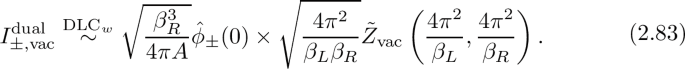
The second factor is exactly the dual-channel vacuum term of the partition function \(\tilde{Z}\). It is known in [28] \(\frac{\tilde{Z}_{T\leqslant h\leqslant A-\varepsilon }(\beta _L,\beta _R)}{\sqrt{\frac{4\pi ^2}{\beta _{L}\beta _{R}}}\tilde{Z}_\textrm{vac}\left( \frac{4\pi ^2}{\beta _{L}},\frac{4\pi ^2}{\beta _{R}}\right) }\) and \(\frac{\tilde{Z}_{h\geqslant A+\varepsilon }(\beta _L,\beta _R)}{\sqrt{\frac{4\pi ^2}{\beta _{L}\beta _{R}}}\tilde{Z}_\textrm{vac}\left( \frac{4\pi ^2}{\beta _{L}},\frac{4\pi ^2}{\beta _{R}}\right) }\) decays exponentially fast in the M\(^*\) limit. The DLC\(_w\) limit in this paper is a stronger version of the M\(^*\) limit, and it is sufficient to kill the extra slow-growing factors \(\beta _{R}^{-3/2}\).
For the explicit constructions and technical details, see [50], Eqs. (38)–(42) and appendix C.
We anticipate that (3.3) can be derived by imposing a similar, yet stronger, sparseness condition compared to the HKS sparseness condition introduced in [22]. While the HKS condition focuses on the sparseness of the low-energy spectrum, (3.3) specifically requires sparseness in the low-twist spectrum.
One can verify the black hole thermodynamics: \(dM=T_{\textrm{H}:} dS+\Omega dJ\).
Corollary 3.3 predicts \(S\approx 2\pi \sqrt{\frac{c-1}{6}J}\) instead of \(2\pi \sqrt{\frac{c}{6}J}\). This is because in this paper we are only counting Virasoro primaries instead of all states. This gap can be filled when we take into account Virasoro descendants. Also, in the large central charge limit, this difference is not important in the leading order of \(c^{-1}\).
We modify the condition stated in ref. [60], Eq. (2.14), to \(J=O(c^3)\). We believe this to be the correct equivalent condition to \(\beta _{R}=O(c^{-1})\). The reason will become clear shortly: We will see that \(\beta _{R}=2\pi \sqrt{\frac{A}{J}}\) under the saddle point approximation. This identification, along with the condition \(\beta _{R}=O(c^{-1})\), implies \(J=O(c^3)\). This has also been noted in Appendix B of [75] to justify the validity of saddle.
By definition, we have \(\hat{\phi }_{+}(0)>0\), whereas it is not always the case that \(\hat{\phi }_{-}(0)\ne 0\) (see the defining properties of \(\phi _{\pm }\) in (2.36)) and (2.37). In this paper, we will explicitly choose a specific form of \(\phi _\pm \) that ensures \(\hat{\phi }_{\pm }(0)\ne 0\).

References
Cardy, J.L.: Operator content of two-dimensional conformally invariant theories. Nucl. Phys. B 270, 186–204 (1986). https://doi.org/10.1016/0550-3213(86)90552-3
Verlinde, E.P.: On the Holographic Principle in a Radiation Dominated Universe. ar**v:hep-th/0008140
Kutasov, D., Larsen, F.: Partition sums and entropy bounds in weakly coupled CFT. JHEP 01, 001 (2001). https://doi.org/10.1088/1126-6708/2001/01/001
Shaghoulian, E.: Modular forms and a generalized Cardy formula in higher dimensions. Phys. Rev. D 93(12), 126005 (2016). https://doi.org/10.1103/PhysRevD.93.126005
Kraus, P., Maloney, A.: A Cardy formula for three-point coefficients or how the black hole got its spots. JHEP 05, 160 (2017). https://doi.org/10.1007/JHEP05(2017)160
Das, D., Datta, S., Pal, S.: Charged structure constants from modularity. JHEP 11, 183 (2017). https://doi.org/10.1007/JHEP11(2017)183
Das, D., Datta, S., Pal, S.: Universal asymptotics of three-point coefficients from elliptic representation of Virasoro blocks. Phys. Rev. D 98(10), 101901 (2018). https://doi.org/10.1103/PhysRevD.98.101901
Cardy, J., Maloney, A., Maxfield, H.: A new handle on three-point coefficients: OPE asymptotics from genus two modular invariance. JHEP 10, 136 (2017). https://doi.org/10.1007/JHEP10(2017)136
Brehm, E.M., Das, D., Datta, S.: Probing thermality beyond the diagonal. Phys. Rev. D 98(12), 126015 (2018). https://doi.org/10.1103/PhysRevD.98.126015
Collier, S., Maloney, A., Maxfield, H., Tsiares, I.: Universal dynamics of heavy operators in CFT\(_{2}\). JHEP 07, 074 (2020). https://doi.org/10.1007/JHEP07(2020)074
Pal, S., Sun, Z.: High energy modular bootstrap, global symmetries and defects. JHEP 08, 064 (2020). https://doi.org/10.1007/JHEP08(2020)064
Harlow, D., Ooguri, H.: A universal formula for the density of states in theories with finite-group symmetry. Class. Quant. Grav. 39(13), 134003 (2022). https://doi.org/10.1088/1361-6382/ac5db2
Belin, A., de Boer, J., Liska, D.: Non-Gaussianities in the statistical distribution of heavy OPE coefficients and wormholes. JHEP 06, 116 (2022). https://doi.org/10.1007/JHEP06(2022)116
Anous, T., Belin, A., de Boer, J., Liska, D.: OPE statistics from higher-point crossing. JHEP 06, 102 (2022). https://doi.org/10.1007/JHEP06(2022)102
Lin, Y.-H., Okada, M., Seifnashri, S., Tachikawa, Y.: Asymptotic density of states in 2d CFTs with non-invertible symmetries. JHEP 03, 094 (2023). https://doi.org/10.1007/JHEP03(2023)094
Benjamin, N., Lee, J., Ooguri, H., and Simmons-Duffin, D.: Universal Asymptotics for High Energy CFT Data. ar**v:2306.08031
Strominger, A., Vafa, C.: Microscopic origin of the Bekenstein–Hawking entropy. Phys. Lett. B 379, 99–104 (1996). https://doi.org/10.1016/0370-2693(96)00345-0
Strominger, A.: Black hole entropy from near horizon microstates. JHEP 02, 009 (1998). https://doi.org/10.1088/1126-6708/1998/02/009
Sen, A.: Black hole entropy function, attractors and precision counting of microstates. Gen. Rel. Grav. 40, 2249–2431 (2008). https://doi.org/10.1007/s10714-008-0626-4
Hellerman, S.: A universal inequality for CFT and quantum gravity. JHEP 08, 130 (2011). https://doi.org/10.1007/JHEP08(2011)130
Sen, A.: Logarithmic corrections to Schwarzschild and other non-extremal black hole entropy in different dimensions. JHEP 04, 156 (2013). https://doi.org/10.1007/JHEP04(2013)156
Hartman, T., Keller, C.A., Stoica, B.: Universal spectrum of 2d conformal field theory in the large c limit. JHEP 09, 118 (2014). https://doi.org/10.1007/JHEP09(2014)118
Mukhametzhanov, B., Zhiboedov, A.: Modular invariance, Tauberian theorems and microcanonical entropy. JHEP 10, 261 (2019). https://doi.org/10.1007/JHEP10(2019)261
Pal, S., Sun, Z.: Tauberian–Cardy formula with spin. JHEP 01, 135 (2020). https://doi.org/10.1007/JHEP01(2020)135
Korevaar, J.: Tauberian theory: a century of developments. Springer (2004). https://doi.org/10.1007/978-3-662-10225-1
Pappadopulo, D., Rychkov, S., Espin, J., Rattazzi, R.: OPE convergence in conformal field theory. Phys. Rev. D 86, 105043 (2012). https://doi.org/10.1103/PhysRevD.86.105043
Qiao, J., Rychkov, S.: A Tauberian theorem for the conformal bootstrap. JHEP 12, 119 (2017). https://doi.org/10.1007/JHEP12(2017)119
Pal, S., Qiao, J., Rychkov, S.: Twist accumulation in conformal field theory. A rigorous approach to the lightcone bootstrap. Commun. Math. Phys. (2023). https://doi.org/10.1007/s00220-023-04767-w
Collier, S., Lin, Y.-H., Yin, X.: Modular bootstrap revisited. JHEP 09, 061 (2018). https://doi.org/10.1007/JHEP09(2018)061
Kusuki, Y.: Light cone bootstrap in general 2D CFTs and entanglement from light cone singularity. JHEP 01, 025 (2019). https://doi.org/10.1007/JHEP01(2019)025
Collier, S., Gobeil, Y., Maxfield, H., Perlmutter, E.: Quantum Regge trajectories and the Virasoro analytic bootstrap. JHEP 05, 212 (2019). https://doi.org/10.1007/JHEP05(2019)212
Benjamin, N., Ooguri, H., Shao, S.-H., Wang, Y.: Light-cone modular bootstrap and pure gravity. Phys. Rev. D 100(6), 066029 (2019). https://doi.org/10.1103/PhysRevD.100.066029
Afkhami-Jeddi, N., Colville, K., Hartman, T., Maloney, A., Perlmutter, E.: Constraints on higher spin CFT\(_{2}\). JHEP 05, 092 (2018). https://doi.org/10.1007/JHEP05(2018)092
Di Francesco, P., Mathieu, P., Senechal, D.: Conformal Field Theory. Graduate Texts in Contemporary Physics. Springer-Verlag, New York (1997)
Antunes, A., Behan, C.: Coupled minimal conformal field theory models revisited. Phys. Rev. Lett. 130(7), 071602 (2023). https://doi.org/10.1103/PhysRevLett.130.071602
Saad, P., Shenker, S.H., Stanford, D.: A Semiclassical Ramp in SYK and in Gravity. ar**v:1806.06840
Collier, S., Maloney, A.: Wormholes and spectral statistics in the Narain ensemble. JHEP 03, 004 (2022). https://doi.org/10.1007/JHEP03(2022)004. ar**v:2106.12760 [hep-th]
Haehl, F.M., Marteau, C., Reeves, W., Rozali, M.: Symmetries and Spectral Statistics in Chaotic Conformal Field Theories. ar**v:2302.14482
Di Ubaldo, G., Perlmutter, E.: AdS\(_3\)/RMT\(_2\) Duality. ar**v:2307.03707
Benjamin, N., Collier, S., Fitzpatrick, A.L., Maloney, A., Perlmutter, E.: Harmonic analysis of 2d CFT partition functions. JHEP 09, 174 (2021). https://doi.org/10.1007/JHEP09(2021)174. ar**v:2107.10744 [hep-th]
Roberts, D.A., Stanford, D.: Two-dimensional conformal field theory and the butterfly effect. Phys. Rev. Lett. 115(13), 131603 (2015). https://doi.org/10.1103/PhysRevLett.115.131603
Basu, P., Das, D., Datta, S., Pal, S.: Thermality of eigenstates in conformal field theories. Phys. Rev. E 96(2), 022149 (2017). https://doi.org/10.1103/PhysRevE.96.022149
Romero-Bermúdez, A., Sabella-Garnier, P., Schalm, K.: A Cardy formula for off-diagonal three-point coefficients; or, how the geometry behind the horizon gets disentangled. JHEP 09, 005 (2018). https://doi.org/10.1007/JHEP09(2018)005
Hikida, Y., Kusuki, Y., Takayanagi, T.: Eigenstate thermalization hypothesis and modular invariance of two-dimensional conformal field theories. Phys. Rev. D 98(2), 026003 (2018). https://doi.org/10.1103/PhysRevD.98.026003
Haehl, F.M., Rozali, M.: Effective field theory for chaotic CFTs. JHEP 10, 118 (2018). https://doi.org/10.1007/JHEP10(2018)118
Anous, T., Haehl, F.M.: On the Virasoro six-point identity block and chaos. JHEP 08(08), 002 (2020). https://doi.org/10.1007/JHEP08(2020)002
Altland, A., Sonner, J.: Late time physics of holographic quantum chaos. SciPost Phys. 11, 034 (2021). https://doi.org/10.21468/SciPostPhys.11.2.034
Choi, C., Haehl, F.M., Mezei, M., Sárosi, G.: Effective Description of Sub-Maximal Chaos: Stringy Effects for SYK Scrambling. ar**v:2301.05698
Ganguly, S., Pal, S.: Bounds on the density of states and the spectral gap in CFT\(_{2}\). Phys. Rev. D 101(10), 106022 (2020). https://doi.org/10.1103/PhysRevD.101.106022
Mukhametzhanov, B., Pal, S.: Beurling–Selberg extremization and modular bootstrap at high energies. SciPost Phys. 8(6), 88 (2020). https://doi.org/10.21468/SciPostPhys.8.6.088
Maldacena, J., Stanford, D., Yang, Z.: Conformal symmetry and its breaking in two dimensional Nearly Anti-de-Sitter space. PTEP 2016(12), 12C104 (2016). https://doi.org/10.1093/ptep/ptw124. ar**v:1606.01857 [hep-th]
Brown, J.D., Henneaux, M.: Central charges in the canonical realization of asymptotic symmetries: an example from three-dimensional gravity. Commun. Math. Phys. 104, 207–226 (1986). https://doi.org/10.1007/BF01211590
Fitzpatrick, A.L., Kaplan, J., Poland, D., Simmons-Duffin, D.: The analytic bootstrap and AdS Superhorizon locality. JHEP 12, 004 (2013). https://doi.org/10.1007/JHEP12(2013)004. ar**v:1212.3616 [hep-th]
Komargodski, Z., Zhiboedov, A.: Convexity and liberation at large spin. JHEP 11, 140 (2013). https://doi.org/10.1007/JHEP11(2013)140. ar**v:1212.4103 [hep-th]
Mukhametzhanov, B., Zhiboedov, A.: Analytic Euclidean bootstrap. JHEP 10, 270 (2019). https://doi.org/10.1007/JHEP10(2019)270. ar**v:1808.03212 [hep-th]
Benjamin, N., Collier, S., Maloney, A.: Pure gravity and conical defects. JHEP 09, 034 (2020). https://doi.org/10.1007/JHEP09(2020)034. ar**v:2004.14428 [hep-th]
Selberg, A.: Collected Papers, vol.2, Lectures on Sieves, Chapter 20. Springer-Verlag, Berlin Heidelberg (1991). https://springer.longhoe.net/book/9783642410222
Littmann, F.: Quadrature and extremal bandlimited functions. SIAM J. Math. Anal. 45(2), 732–747 (2013). https://doi.org/10.1137/120888004
Beurling, A.: The Collected Works of Arne Beurling. Contemporary Mathematicians. Birkhäuser, Boston (1989)
Ghosh, A., Maxfield, H., Turiaci, G.J.: A universal Schwarzian sector in two-dimensional conformal field theories. JHEP 05, 104 (2020). https://doi.org/10.1007/JHEP05(2020)104. ar**v:1912.07654 [hep-th]
Banados, M., Teitelboim, C., Zanelli, J.: The Black hole in three-dimensional space-time. Phys. Rev. Lett. 69, 1849–1851 (1992). https://doi.org/10.1103/PhysRevLett.69.1849. ar**v:hep-th/9204099
Hyun, S., Lee, G.H., Yee, J.H.: Hawking radiation from (2+1)-dimensional black hole. Phys. Lett. B 322, 182–187 (1994). https://doi.org/10.1016/0370-2693(94)91104-5
Ichinose, I., Satoh, Y.: Entropies of scalar fields on three-dimensional black holes. Nucl. Phys. B 447, 340–372 (1995). https://doi.org/10.1016/0550-3213(95)00197-Z
Carlip, S., Teitelboim, C.: Aspects of black hole quantum mechanics and thermodynamics in (2+1)-dimensions. Phys. Rev. D 51, 622–631 (1995). https://doi.org/10.1103/PhysRevD.51.622
Brown, J.D., Creighton, J., Mann, R.B.: Temperature, energy and heat capacity of asymptotically anti-de Sitter black holes. Phys. Rev. D 50, 6394–6403 (1994). https://doi.org/10.1103/PhysRevD.50.6394
Carlip, S.: The (2+1)-dimensional black hole. Class. Quant. Grav. 12, 2853–2880 (1995). https://doi.org/10.1088/0264-9381/12/12/005
Carlip, S., Gegenberg, J., Mann, R.B.: Black holes in three-dimensional topological gravity. Phys. Rev. D 51, 6854–6859 (1995). https://doi.org/10.1103/PhysRevD.51.6854
Englert, F., Reznik, B.: Entropy generation by tunneling in (2+1) gravity. Phys. Rev. D 50, 2692–2699 (1994). https://doi.org/10.1103/PhysRevD.50.2692
Medved, A.J.M.: Radiation via tunneling in the charged BTZ black hole. Class. Quant. Grav. 19, 589–598 (2002). https://doi.org/10.1088/0264-9381/19/3/313
Emparan, R., Sachs, I.: Quantization of AdS(3) black holes in external fields. Phys. Rev. Lett. 81, 2408–2411 (1998). https://doi.org/10.1103/PhysRevLett.81.2408
Preskill, J., Schwarz, P., Shapere, A.D., Trivedi, S., Wilczek, F.: Limitations on the statistical description of black holes. Mod. Phys. Lett. A 6, 2353–2362 (1991). https://doi.org/10.1142/S0217732391002773
Landau, L.D., Lifshitz, E.M.: Statistical Physics, vol. 5. Elsevier (2013)
Turiaci, G.J.: New Insights on Near-Extremal Black Holes. ar**v:2307.10423
Mertens, T.G., Turiaci, G.J., Verlinde, H.L.: Solving the Schwarzian via the conformal bootstrap. JHEP 08, 136 (2017). https://doi.org/10.1007/JHEP08(2017)136
Aggarwal, A., Castro, A., Detournay, S., Mühlmann, B.: Near-Extremal Limits of Warped CFTs. ar**v:2211.03770
Heydeman, M., Iliesiu, L.V., Turiaci, G.J., Zhao, W.: The statistical mechanics of near-BPS black holes. J. Phys. A 55(1), 014004 (2022). https://doi.org/10.1088/1751-8121/ac3be9
Iliesiu, L.V., Murthy, S. Turiaci, G.J.: Black Hole Microstate Counting from the Gravitational Path Integral. ar**v:2209.13602
Iliesiu, L.V., Murthy, S., Turiaci, G.J.: Revisiting the Logarithmic Corrections to the Black Hole Entropy. ar**v:2209.13608
Lin, Y.-H., Shao, S.-H.: \({{\mathbb{Z} }}_N\) symmetries, anomalies, and the modular bootstrap. Phys. Rev. D 103(12), 125001 (2021). https://doi.org/10.1103/PhysRevD.103.125001
Lin, Y.-H., Shao, S.-H.: Bootstrap** Non-invertible Symmetries. ar**v:2302.13900
Kang, M.J., Lee, J., Ooguri, H.: Universal formula for the density of states with continuous symmetry. Phys. Rev. D 107(2), 026021 (2023). https://doi.org/10.1103/PhysRevD.107.026021
Choi, Y., Rayhaun, B.C., Sanghavi, Y., Shao, S.-H.: Comments on Boundaries, Anomalies, and Non-Invertible Symmetries. ar**v:2305.09713
Maxfield, H.: Quantum corrections to the BTZ black hole extremality bound from the conformal bootstrap. JHEP 12, 003 (2019). https://doi.org/10.1007/JHEP12(2019)003
Chandra, J., Hartman, T.: Toward Random Tensor Networks and Holographic Codes in CFT. ar**v:2302.02446
Chandra, J.: Euclidean Wormholes for Individual 2d CFTs. ar**v:2305.07183
Acknowledgements
We thank Nathan Benjamin, Gabriele Di Ubaldo, Tom Hartman, Yikun Jiang, João Penedones, Eric Perlmutter, Biswajit Sahoo, Joaquin Turiaci and Yang Zhou for useful and enlightening discussions. We also thank Alexandre Belin, João Penedones, Slava Rychkov and Joaquin Turiaci for useful comments on the draft. SP acknowledges the support by the U.S. Department of Energy, Office of Science, Office of High Energy Physics, under Award Number DE-SC0011632 and by the Walter Burke Institute for Theoretical Physics. JQ is supported by the Swiss National Science Foundation through the National Centre of Competence in Research SwissMAP and by the Simons Foundation grant 994302 (Simons Collaboration on Confinement and the QCD Strings).
Funding
Open access funding provided by EPFL Lausanne.
Author information
Authors and Affiliations
Corresponding author
Additional information
Communicated by Katrin Wendland.
Publisher's Note
Springer Nature remains neutral with regard to jurisdictional claims in published maps and institutional affiliations.
Appendices
Estimating the Dual-Vacuum Term
In this section, we compute the asymptotic behavior of the integral
in the modular double lightcone limit, where
By definition, \(I^{\textrm{dual}}_{\pm ,\mathrm vac}\) is factorized into two parts
When \(\beta _L\rightarrow \infty \), the asymptotic behavior of \(I^\textrm{dual,L}_{\pm ,\mathrm vac}\) is given by
For \(I^{\textrm{dual,R}}_{\pm ,\mathrm vac}\), we introduce the identity
where the kernel \(\rho _0\) is given by
Then, by Eqs. (A.3) and (A.5) we get
We choose \(\phi _\pm \) which satisfy the following properties
Below we will study \(I^{\textrm{dual,R}}_{\pm ,\mathrm vac}(A,\bar{H};\beta _R)\) with \(\beta _R=2\pi \sqrt{\frac{A}{\bar{H}-A}}\) in the limit
We split the kernel \(\rho _0\) in (A.6) into four parts
Correspondingly, \(I^{\textrm{dual,R}}_{\pm ,\mathrm vac}\) is split into four parts
We would like to show that for \(\hat{\phi }_\pm (0)\ne 0\)Footnote 17:
In the limit (A.9), the dominant contribution to \(I^{\textrm{dual,R}}_{\pm ,\mathrm vac}\) comes from \(I^{R(1)}_{\pm ,\mathrm vac}\). Consequently, \(I^{\textrm{dual}}_{\pm ,\mathrm vac}\) has the following asymptotic behavior:
where the r.h.s. corresponds to the contribution from \(I^{R(1)}_{\pm ,\mathrm vac}\), which will be derived in the next subsection.
1.1 Estimating \(I^{R(1)}_{\pm ,\mathrm vac}\) (the Dominant Term)
By definition, \(I^{R(1)}_{\pm ,\mathrm vac}\) is given by
We rewrite \(I^{R(1)}_{\pm ,\mathrm vac}\) as
We split the domain of integration into two parts
where \(\tau \in (\frac{1}{2},1)\) is some fixed constant. The first integral is bounded by
Here, we bounded the exponential factor by 1 and bounded \(\phi _{\pm }\) by its maximal value. Since \(\phi _{\pm }\) has the upper bound (A.8), we get
in the limit (A.9).
The second integral is controlled as follows. We rewrite the integral as
We have
for \(\bar{H}\geqslant \max \left\{ 4A,4^{1/(1-\tau )}\right\} \). Let us explain the above bound. Since \(\bar{H}\geqslant \max \left\{ 4A,4^{1/(1-\tau )}\right\} \), we have \({\bar{H}}\geqslant 4A\) and \(\bar{H} \geqslant 4 {\bar{H}}^\tau \), leading to \({\bar{H}}-A-{\bar{H}}^\tau \geqslant {\bar{H}}/2\). Plugging this in, we obtain \(\sqrt{\frac{\bar{H}}{\bar{H}-\bar{H}^\tau -A}}\leqslant \sqrt{2}\).
Now, the exponential factor in \(Y_{\bar{H}}(x)\) is obviously bounded by 1. So we get \(|Y_{\bar{H}}(x)|\leqslant \sqrt{2}|\phi _\pm (x)|\) for sufficiently large \(\bar{H}\) and the r.h.s. is an integrable function on \(\mathbb {R}\). Now, we consider the point-wise limit of \(Y_{\bar{H}}(x)\) as \(\bar{H}\) goes to \(\infty \). First, using \(\tau >0\) we have
for fixed x. With the choice \(\beta _R=2\pi \sqrt{\frac{A}{\bar{H}-A}}\), which gives
for fixed x in the limit (A.9). Thus, we get \(Y_{\bar{H}}(x){\mathop {\longrightarrow }\limits ^{(A.9)}}\phi _\pm (x)\) for fixed x. Then, using the dominated convergence theorem we conclude that
Putting everything together, we get
1.2 Estimating \(I^{R(2)}_{\pm ,\mathrm vac}\)
By definition, \(I^{R(2)}_{\pm ,\mathrm vac}\) is given by
Similarly to the analysis for \(I^{R(1)}_{\pm ,\mathrm vac}\), we rewrite \(I^{R(2)}_{\pm ,\mathrm vac}\) as
We see that its structure is very similar to (A.14), except that A is replaced by \(A-1\) in two places. Then, we do the same analysis as \(I^{R(1)}_{\pm ,\mathrm vac}\). We split the domain of integration into two parts as we have done in (A.15). Here, the analysis is simpler than \(I^{R(1)}_{\pm ,\mathrm vac}\): In the integrand, we always bound the exponential factor by 1. In the limit (A.9), the main difference here is the exponential factor \(e^{\frac{4\pi ^2 (A-1)}{\beta _R}}\) which grows slower than \(e^{\frac{4\pi ^2 A}{\beta _R}}\) (which is the one in \(I^{R(1)}_{\pm ,\mathrm vac}\)) as \(\beta _{R}\rightarrow 0\). Then in limit (A.9) (with \(\beta _R=2\pi \sqrt{\frac{A}{\bar{H}-A}}\)) we have
because of the exponential suppression. Here, the notation “\(const(\phi _\pm )\)” means some finite constant which depends on the choice of \(\phi _\pm \).
1.3 Estimating \(I^{R(3)}_{\pm ,\mathrm vac}\) and \(I^{R(4)}_{\pm ,\mathrm vac}\)
By definition, \(I^{R(3)}_{\pm ,\mathrm vac}\) is given by
Similarly to the analysis for \(I^{R(1)}_{\pm ,\mathrm vac}\), we rewrite \(I^{R(3)}_{\pm ,\mathrm vac}\) as
We see that \(I^{R(3)}_{\pm ,\mathrm vac}\) only differs from \(I^{R(1)}_{\pm ,\mathrm vac}\) by a change of the “±” sign in the exponential factor. Then, the analysis is similar to \(I^{R(1)}_{\pm ,\mathrm vac}\). We split the integral into two parts as we have done in (A.15). In the limit (A.9), the first part goes to zero for the same reason, and the second part is controlled by the dominated convergence theorem. But for \(I^{R(3)}_{\pm ,\mathrm vac}\) we have
Here in the first line, we used \(\beta _R=2\pi \sqrt{\frac{A}{\bar{H}-A}}\), in the second line we dropped the first term in the bracket, and in the last line used (A.9). This estimate implies that the second part of the integral also goes to zero. Therefore, we get
By the same analysis, we can also get
So we conclude that \(I^{R(3)}_{\pm ,\mathrm vac}\) and \(I^{R(4)}_{\pm ,\mathrm vac}\) are subleading in the limit (A.9).
Some Uniform Bounds on \(\phi _{\pm ,\delta }\)
In this appendix, we address the subtleties that arise when we take the limit \(\delta \rightarrow 0\) or \(\delta \rightarrow 1\) for the selected functions \(\phi _{\pm ,\delta }\) (as discussed in Sect. 2.8, specifically points 1 and 2). Throughout our analysis, we consistently choose the following expressions for \(\phi _{\pm ,\delta }\), which are (2.96) rescaled under (2.98):
Recall that the range of allowed values for \(\delta \) is given by \(\varepsilon<\delta <1-\varepsilon \). As we approach the limit \(\varepsilon \rightarrow 0\), it eventually leads us to consider \(\delta \rightarrow 0\) for \(\phi _{+,\delta }\) and \(\delta \rightarrow 1\) for \(\phi _{-,\delta }\). In these limits, the values of the corresponding functions \(\phi _{\pm ,\delta }\) are obtained point-wise as follows:
These limits are well-defined functions and are \(L^1\)-integrable over the real axis. This observation provides strong evidence that \(\phi _{\pm ,\delta }\) satisfy certain uniform bounds that are essential for our analysis.
We aim to establish the following properties of \(\phi _{\pm ,\delta }\):
Lemma 1
For a fixed \(\Lambda \in (0,2\pi ]\), the function \(\phi _{+,\delta }\) satisfies the following bounds for \(\delta \in \left[ 0,\frac{1}{2}\right] \):
Lemma 2
Let \(w\in \left( \frac{1}{2},1\right) \) and \(\Lambda \in \left[ \frac{(2w+1)\pi }{2},2\pi w\right] \) be fixed. For \(\delta \in \left[ \frac{(2w+1)\pi }{2\Lambda },1\right] \), the function \(\phi _{-,\delta }\) satisfies the following bounds:
1.1 Proof of Lemma 1
When \(\left|x\right|\geqslant 1\), we have
In the first step, we rewrite \(\phi _{+,\delta }(x)\). In the second step, we bound \(\sin \) and \(\cos \) by 1 and use the fact that \(\frac{\sin (\delta \Lambda )}{\delta \Lambda }\geqslant 0\) for \(\delta \in \left[ 0,\frac{1}{2}\right] \) and \(\Lambda \in (0,2\pi ]\). In the last step, we use the fact that \(|x|-\delta \geqslant \frac{|x|}{2}\) for \(|x|\geqslant 1\) and \(\delta \in \left[ 0,\frac{1}{2}\right] \).
When \(0\leqslant x\leqslant 1\), we have
In the first step, we rewrite \(\phi _{+,\delta }(x)\). In the second step, we use the inequality \(|\frac{\sin x}{x}|\leqslant 1\) for any \(x\in \mathbb {R}\) and \(\sin x\leqslant x\) for \(x\geqslant 0\). In the last step, we use the fact that \(\frac{\sin (\delta \Lambda )}{\delta \Lambda }\geqslant 0\) for \(\delta \in \left[ 0,\frac{1}{2}\right] \) and \(\Lambda \in (0,2\pi ]\). The same bound on \(\phi _{+,\delta }(x)\) holds for \(-1\leqslant x\leqslant 0\) because it is an even function of x. This completes the proof of the first inequality in (B.3). Next, we derive a uniform upper bound on the ratio \(\left|\frac{\phi _{+,\delta }(x)}{\hat{\phi }_{+,\delta }(0)}\right|\). Using (2.100), we have \(\hat{\phi }_{+,\delta }(0)\geqslant \frac{1}{\Lambda }\) for \(\Lambda \in (0,2\pi ]\) and \(\delta \in \left[ 0,\frac{1}{2}\right] \). Together with the first inequality in (B.3), we obtain
The bound on \(|\frac{\hat{\phi }{+,\delta }(x)}{\hat{\phi }{+,\delta }(0)}|\) follows trivially from the fact that \(\phi {+,\delta }(x)\geqslant 0\) for all x. Hence, we have \(\left|\frac{\hat{\phi }_{+,\delta }(x)}{\hat{\phi }_{+,\delta }(0)}\right|\leqslant 1.\) This completes the proof of Lemma 1.
1.2 Proof of Lemma 2
We note that \(\phi _{-,\delta }(x)\) is an even function of x, so it is sufficient to prove the first inequality in (B.4) for \(x\geqslant 0\). We rewrite \(\phi _{-,\delta }(x)\) as follows:
When \(x\geqslant 0\), the first factor in (B.8) is bounded by 1. For the second factor, we use the condition on the range of \(\delta \) and \(\Lambda \), which implies that \(\frac{\delta \Lambda }{2}\in \left[ \frac{\pi }{2},\pi \right] \). Thus, the second factor is bounded as follows \(G_1\leqslant \frac{\pi ^2}{\Lambda ^2}\) where we used the fact that the function \(f(x)\equiv (\cos x-\frac{\sin x}{x})^{-2}\) is maximized at \(x=\frac{\pi }{2}\) with the maximum value of \(\frac{\pi ^2}{4}\) for \(\frac{\pi }{2}\leqslant x\leqslant \pi \). The last factor in (B.8) is bounded as follows \(G_2\leqslant (\frac{\Lambda }{2}+\frac{\Lambda }{2})^2=\Lambda ^2.\) This bound is obtained by using the inequalities \(\left|\frac{\sin x}{x}\right|\leqslant 1\), \(\left|\sin x\right|\leqslant \left|x\right|\), and \(\left|\cos x\right|\leqslant 1\). Combining the inequalities derived above, we obtain \(\left|\phi _{-,\delta }(x)\right|\leqslant \pi ^2\quad (\forall \ x\in \mathbb {R}).\) In particular, this bound holds for \(\left|x\right|\leqslant 2\).
When \(x\geqslant 2\), we use the condition \(\delta \leqslant 1\) and further refine the bound by noting that the last factor in (B.8) satisfies: \(B\leqslant ((x-1)^{-1}+x^{-1})^2\leqslant 4(x-1)^{-2}\). Thus, we obtain the improved bound \(\left|\phi _{-,\delta }(x)\right|\leqslant \frac{4\pi ^2}{\Lambda ^2(\left|x\right|-1)^2}\quad (\left|x\right|\geqslant 2).\) This completes the proof of the first inequality in (B.4).
For the second and third inequalities in (B.4), we make use of the explicit expression of \(\hat{\phi }_{-,\delta }\) given in (2.100):
Here, we used the condition \(\frac{(2w+1)\pi }{4}\leqslant \frac{\delta \Lambda }{2}\leqslant \pi \), where \(\frac{1}{2}< w<1\), and the fact that \(\frac{1}{1-\frac{\tan x}{x}}\) is monotonically increasing for \(\frac{\pi }{2}\leqslant x\leqslant \pi \). Consequently, \(\hat{\phi }_{-,\delta }(0)\) possesses a strictly positive lower bound that remains uniform in \(\delta \) within the specified range.
The second inequality of (B.4) follows from (B.9) and the first inequality of (B.4). Similarly, the third inequality of (B.4) is obtained by combining (B.9) and the first inequality of (B.9) with the additional estimate:
Therefore, we have established the validity of the second and third inequalities in (B.4), completing the proof of Lemma 2.
Rights and permissions
Open Access This article is licensed under a Creative Commons Attribution 4.0 International License, which permits use, sharing, adaptation, distribution and reproduction in any medium or format, as long as you give appropriate credit to the original author(s) and the source, provide a link to the Creative Commons licence, and indicate if changes were made. The images or other third party material in this article are included in the article's Creative Commons licence, unless indicated otherwise in a credit line to the material. If material is not included in the article's Creative Commons licence and your intended use is not permitted by statutory regulation or exceeds the permitted use, you will need to obtain permission directly from the copyright holder. To view a copy of this licence, visit http://creativecommons.org/licenses/by/4.0/.
About this article

Cite this article
Pal, S., Qiao, J. Lightcone Modular Bootstrap and Tauberian Theory: A Cardy-Like Formula for Near-Extremal Black Holes. Ann. Henri Poincaré (2024). https://doi.org/10.1007/s00023-024-01441-2
Received:
Accepted:
Published:
DOI: https://doi.org/10.1007/s00023-024-01441-2