Convergence of an asynchronous block-coordinate forward-backward algorithm for convex composite optimization

Abstract

In this paper, we study the convergence properties of a randomized block-coordinate descent algorithm for the minimization of a composite convex objective function, where the block-coordinates are updated asynchronously and randomly according to an arbitrary probability distribution. We prove that the iterates generated by the algorithm form a stochastic quasi-Fejér sequence and thus converge almost surely to a minimizer of the objective function. Moreover, we prove a general sublinear rate of convergence in expectation for the function values and a linear rate of convergence in expectation under an error bound condition of Tseng type. Under the same condition strong convergence of the iterates is provided as well as their linear convergence rate.

1 Introduction

We consider the composite minimization problem

$$\begin{aligned} \underset{\varvec{\textsf{x}}\in \varvec{{\textsf{H}}}}{\text {minimize }} F(\varvec{\textsf{x}}) := f(\varvec{\textsf{x}}) + g(\varvec{\textsf{x}}),\qquad g(\varvec{\varvec{\textsf{x}}}) := \sum _{i=1}^m g_i(\textsf{x}_i), \end{aligned}$$

(1.1)

where $\varvec{{\textsf{H}}}$ is the direct sum of m separable real Hilbert spaces $(\textsf{H}_i)_{1 \le i \le m}$, that is, $\varvec{{\textsf{H}}}= \bigoplus _{i=1}^{m} \textsf{H}_i$ and the following assumptions are satisfied unless stated otherwise.

• A1 $f :\varvec{{\textsf{H}}}\rightarrow \mathbb {R}$ is convex and differentiable.

• A2 For every $i \in \{1, \ldots , m\}$, $g_i :\textsf{H}_i \rightarrow ]-\infty ,+\infty ]$ is proper convex and lower semicontinuous.

• A3 For all $\varvec{\textsf{x}}\in \varvec{{\textsf{H}}}$ and $i \in \{1, \ldots , m\}$, the map $\nabla f(\textsf{x}_1, \dots ,\textsf{x}_{i-1}, \cdot , \textsf{x}_{i+1}, \dots , \textsf{x}_m): \textsf{H}_i \rightarrow \varvec{{\textsf{H}}}$ is Lipschitz continuous with constant $L_\text {res}>0$ and the map $\nabla _i f(\textsf{x}_1, \dots ,\textsf{x}_{i-1}, \cdot , \textsf{x}_{i+1}, \dots , \textsf{x}_m):\textsf{H}_i \rightarrow \textsf{H}_i$ is Lipschitz continuous with constant $L_i$. Note that $L_{\max }{:}{=}\max _i L_i \le L_\text {res}$ and $L_{\min } {:}{=}\min _i L_i$.

• A4 F attains its minimum $F^*:= \min F$ on $\varvec{{\textsf{H}}}$.

To solve problem 1.1, we use the following asynchronous block-coordinate descent algorithm. It is an extension of the parallel block-coordinate proximal gradient method considered in [42] to the asynchronous setting, where an inconsistent delayed gradient vector may be processed at each iteration.

Algorithm 1.1

Let $(i_k)_{k \in \mathbb {N}}$ be a sequence of i.i.d. random variables with values in $[m]:=\{1, \dots , m\}$ and $\textsf{p}_i$ be the probability of the event $\{i_k = i\}$, for every $i \in [m]$. Let $(\varvec{{\textsf{d}}}^k)_{k \in \mathbb {N}}$ be a sequence of integer delay vectors, $\varvec{{\textsf{d}}}^k = (\textsf{d}_1^k, \dots , \textsf{d}_m^k) \in \mathbb {N}^m$ such that $\max _{1\le i\le m} \textsf{d}^k_i \le \min \{k,\tau \}$ for some $\tau \in \mathbb {N}$. This delay vector is deterministic and independent from the block coordinates selection process $(i_k)_{k \in \mathbb {N}}$. Let $(\gamma _i)_{1 \le i \le m} \in \mathbb {R}_{++}^m$ and $\varvec{x}^0 =(x^0_{1}, \dots , x^0_{m}) \in \varvec{{\textsf{H}}}$ be a constant random variable. Iterate

$$\begin{aligned} \begin{array}{l} \text {for}\;k=0,1,\ldots \\ \left\lfloor \begin{array}{l} \text {for}\;i=1,\dots , m\\ \left\lfloor \begin{array}{l} x^{k+1}_i = {\left\{ \begin{array}{ll} {\textsf {prox}}_{\gamma _{i_{k}} g_{i_{k}}} \big (x^k_{i_{k}} - \gamma _{i_{k}} \nabla _{i_{k}} f (\varvec{x}^{k-\varvec{{\textsf{d}}}^k})\big ) &{}\text {if } i=i_{k}\\ x^k_i &{}\text {if } i \ne i_{k}, \end{array}\right. } \end{array} \right. \end{array} \right. \end{array} \end{aligned}$$

(1.2)

where $\varvec{x}^{k-\varvec{{\textsf{d}}}^k} = (x_1^{k - \textsf{d}^k_1}, \dots , x_m^{k - \textsf{d}^k_m})$.

In this work, we assume the following stepsize rule

$$\begin{aligned} (\forall \, i \in [m])\quad \gamma _i( L_{i} + 2\tau L_{\text {res}}\textsf{p}_{\max }/ \sqrt{\textsf{p}_{\min }})< 2, \end{aligned}$$

(1.3)

where $\textsf{p}_{\max }:= \max _{1 \le i \le m} \textsf{p}_i$ and $\textsf{p}_{\min }:= \min _{1 \le i \le m} \textsf{p}_i$. If there is no delay, namely $\tau = 0$, the usual stepsize rule $\gamma _i < 2/L_i$ is obtained [14, 43].

The presence of the delay vectors in the above algorithm allows to describe a parallel computational model on multiple cores, as we explain below.

1.1 Asynchronous models

In this section we discuss an example of a parallel computational model, occurring in shared-memory system architectures, which can be covered by the proposed algorithm. Consider a situation where we have a machine with multiple cores. They all have access to a shared data $\varvec{x}= (x_1, \dots , x_m)$ and each core updates a block-coordinate $x_i$, $i \in [m]$, asynchronously without waiting for the others. The iteration’s counter k is increased any time a component of $\varvec{x}$ is updated. When a core is given a coordinate to update, it has to read from the shared memory and compute a partial gradient. While performing these two operations, the data $\varvec{x}$ may have been updated by other cores. So, when the core is updating its assigned coordinate at iteration k, the gradient might no longer be up to date. This phenomenon is modelled by using a delay vector $\varvec{{\textsf{d}}}^k$ and evaluating the partial gradient at $\varvec{x}^{k-\varvec{{\textsf{d}}}^k}$ as in Algorithm 1.1. Each component of the delay vector reflects how many times the corresponding coordinate of $\varvec{x}$ have been updated since the core has read this particular coordinate from the shared memory. Note that different delays among the coordinates may arise since the shared data may be updated during the reading phase, so that the partial gradient ultimately is computed at a point which may not be consistent with any past instance of the shared data. This situation is called inconsistent read [6] and, in practice, allows a reading phase without any lock. By contrast, in a consistent read model [30, 39], a lock is put during the reading phase and the delay originates only while computing the partial gradient. The delay is the same for all the block-coordinates, so that the value read by any core is a past instance of the shared data. However, for our theoretical study it does not make any difference considering an inconsistent or a consistent reading setting, because in the end only the maximum delay matters. Inconsistent read model is also considered in [8, 16, 31].

We remark that, in our setting, for all $k \in \mathbb {N}$, the delay vector $\varvec{{\textsf{d}}}^k$ is considered to be a parameter that does not dependent on the random variable $i_k$, similarly to the works [16, 23, 30, 31]. In this way, the stochastic attribute of the sequence $(\varvec{x}_k)_{k \in \mathbb {N}}$ is not determined by the delay, but it only comes from the stochastic selection of the block-coordinates. Some papers consider the case where the delay vector is a stochastic variable that may depend on $i_k$ [8, 45] or that it is unbounded [23, 45]. Those setting are natural extensions to our work that we are considering for future work. Finally, a completely deterministic model, both in the block’s selection and delays is studied in [12].

1.2 Related work

The topic of parallel asynchronous algorithm is not a recent one. In 1969, Chazan and Miranker [9] presented an asynchronous method for solving linear equations. Later on, Bertsekas and Tsitsiklis [6] proposed an inconsistent read model of asynchronous computation. Due to the availability of large amount of data and the importance of large scale optimization, in recent years we have witnessed a surge of interest in asynchronous algorithms. They have been studied and adapted to many optimization problems and methods such as stochastic gradient descent [1, 20, 29, 39, 40], randomized Kaczmarz algorithm [32], and stochastic coordinate descent [2, 30, 41, 45, 51].

In general, stochastic algorithms can be divided in two classes. The first one is when the function f is an expectation i.e., $f(\textsf{x}) = {\textsf{E}}[h(\textsf{x}; \xi )]$. At each iteration k only a stochastic gradient $\nabla h(\cdot ; \xi _k)$ is computed based on the current sample $\xi _k$. In this setting, many asynchronous versions have been proposed, where delayed stochastic gradients are considered, see [3, 10, 20, 28, 34, 36]. The second class, which is the one we studied, is that of randomized block-coordinate methods. Below we describe the related literature.

The work [31] studied a problem and a model of asynchronicity which is similar to ours, but the proposed algorithm AsySPCD requires that the random variables $(i_k)_{k \in \mathbb {N}}$ are uniformly distributed (i.e, $\textsf{p}_i =1/m$) and that the stepsize is the same for all the block-coordinates. This latter assumption is an important limitation, since it does not exploit the possibility of adapting the stepsizes to the block-Lipschitz constants of the partial gradients, hence allowing longer steps along block-coordinates. A linear rate of convergence is also obtained by exploiting a quadratic growth condition which is essentially equivalent to our error bound condition [18]. For a discussion on the limitations of [31] and the improvements we bring, see Remark 3.2 point (vi) and Sect. 6 on numerical experiments.

In the nonconvex case, [16] considers an asynchronous algorithm which may select the blocks both in an almost cyclic manner or randomly with a uniform probability. In the latter case, it is proved that the cluster points of the sequence of the iterates are almost surely stationary points of the objective function. However, the convergence of the whole sequence is not provided, nor is given any rate of convergence for the function values. Moreover, under the Kurdyka-Łojasiewicz (KL) condition [7, 18], linear convergence is also derived, but it is restricted to the deterministic case.

To conclude, we note that our results, when specialized to the case of zero delays, fully recover the ones given in [42].

1.3 Contributions

The main contributions of this work are summarized below:

• We first prove the almost sure weak convergence of the iterates $(\varvec{x}^k)_{k \in \mathbb {N}}$, generated by Algorithm 1.1, to a random variable $\varvec{x}^*$ taking values in ${{\,\mathrm{\mathrm {{argmin}}}\,}}F$. At the same time, we prove a sublinear rate of convergence of the function values in expectation, i.e, $\displaystyle {\textsf{E}}[F(\varvec{x}^k)] - \min F = o(1/k)$. We also provide for the same quantity an explicit rate of $\mathcal {O}(1/k)$, see Theorem 3.1.

• Under an error bound condition of Luo-Tseng type, on top of the strong convergence a.s. of the iterates, we prove linear convergence in expectation of the function values and in mean of the iterates, see Theorem 4.2.

We improve the state-of-the-art under several aspects: we consider an arbitrary probability for the selection of the blocks; the adopted stepsize rule improves over the existing ones, and coincides with the one in [16] in the special case of uniform selection of the blocks—in particular, it allows for larger stepsizes when the number of blocks grows; the almost sure convergence of the iterates in the convex and stochastic setting is new and relies on a stochastic quasi-Fejerian analysis; linear convergence under an error bound condition is also new in the asynchronous stochastic scenario.

The rest of the paper is organized as follows. In the next subsection we set up basic notation. In Sect. 2 we recall few facts and we provide some preliminary results. The general convergence analysis is given in Sect. 3 where the main Theorem 3.1 is presented. Section 4 contains the convergence theory under an additional error bound condition, while applications are discussed in Sect. 5. The majority of proofs are postponed to Appendices 1 and 2.

1.4 Notation

We set $\mathbb {R}_+ = [0,+\infty [$ and $\mathbb {R}_{++} = \; ]0, +\infty [$. For every integer $\ell \ge 1$ we define $[\ell ] = \{1, \dots , \ell \}$. For all $i \in [m]$, we denote indifferently the scalar products of $\varvec{{\textsf{H}}}$ and $\textsf{H}_i$ by $\langle \cdot , \cdot \rangle$ and:

$$\begin{aligned} (\forall \varvec{\varvec{\textsf{x}}} =(\textsf{x}_1, \ldots , \textsf{x}_m), \varvec{\varvec{\textsf{y}}} =(\textsf{y}_1, \ldots , \text {y}_m) \in \varvec{{\textsf{H}}}) \quad \langle \varvec{\varvec{\textsf{x}}}, \varvec{\varvec{\textsf{y}}} \rangle = \sum _{i=1}^{m} \langle \textsf{x}_i, \textsf{y}_i \rangle . \end{aligned}$$

$\Vert \cdot \Vert$ and $|\cdot |$ represent the norms associated to their scalar product in $\varvec{{\textsf{H}}}$ and in any of $\textsf{H}_i$ respectively. We also consider the canonical embedding, for all $i = 1,2, \ldots , m$, ${\textsf{J}}_i:\textsf{H}_i \rightarrow \varvec{{\textsf{H}}}$, $\textsf{x}_i \mapsto (0,\ldots , 0, \textsf{x}_i,0,\ldots ,0)$, with $x_i$ in the $i^{th}$ position. Random vectors and variables are defined on the underlying probability space $(\Omega , \mathfrak {A}, {\textsf{P}})$. The default font is used for random variables while sans serif font is used for their realizations or deterministic variables. Let $(\alpha _i)_{1 \le i \le m} \in \mathbb {R}^m_{++}$. The direct sum operator ${{\textsf{A}}}= \bigoplus _{i=1}^m \alpha _i \textsf{Id}_i$, where $\textsf{Id}_i$ is the identity operator on $\textsf{H}_i$, is

$$\begin{aligned} {{\textsf{A}}}:\varvec{{\textsf{H}}}&\rightarrow \varvec{{\textsf{H}}}\\ \varvec{\textsf{x}}=(\textsf{x}_i)_{1 \le i \le m}&\mapsto (\alpha _i \textsf{x}_i)_{1 \le i \le m} \end{aligned}$$

This operator defines an equivalent scalar product on $\varvec{{\textsf{H}}}$ as follows

$$\begin{aligned} (\forall \, \varvec{\textsf{x}}\in \varvec{{\textsf{H}}})(\forall \, \varvec{\textsf{y}}\in \varvec{{\textsf{H}}})\qquad \langle \varvec{\textsf{x}}, \varvec{\textsf{y}}\rangle _{{{\textsf{A}}}} = \langle {{\textsf{A}}}\varvec{\textsf{x}}, \varvec{\textsf{y}}\rangle = \sum _{i=1}^m \alpha _i \langle \textsf{x}_i, \textsf{y}_i\rangle , \end{aligned}$$

which gives the norm $\Vert \varvec{\textsf{x}}\Vert _{{{\textsf{A}}}}^2 = \sum _{i=1}^m \alpha _i |\textsf{x}_i|^2$. We let

where for all $i \in [m]$, $\gamma _i$ and $\textsf{p}_i$ are defined in Algorithm 1.1. We set $\textsf{p}_{\max }:=\max _{1 \le i \le m} \textsf{p}_{i}$ and $\textsf{p}_{\min }:=\min _{1 \le i \le m} \textsf{p}_{i}.$ Let ${\varphi }:\varvec{{\textsf{H}}}\rightarrow ]-\infty ,+\infty ]$ be proper, convex, and lower semicontinuous. The domain of ${\varphi }$ is ${{\,\mathrm{\text {{dom}}}\,}}{\varphi }= \{\varvec{\textsf{x}}\in \textsf{H}\,\vert \, {\varphi }(\varvec{\textsf{x}})<+\infty \}$ and the set of minimizers of ${\varphi }$ is ${{\,\mathrm{\mathrm {{argmin}}}\,}}{\varphi }= \{\varvec{\textsf{x}}\in \varvec{{\textsf{H}}}\,\vert \, {\varphi }(\varvec{\textsf{x}}) = \inf {\varphi }\}$. We recall that the proximity operator of $\varphi$ is ${\textsf {prox}}_{\varphi }(\varvec{x}) = {{\,\mathrm{\mathrm {{argmin}}}\,}}_{\varvec{y}\in \varvec{{\textsf{H}}}} \varphi (\varvec{y}) + \frac{1}{2} \Vert \varvec{y}-\varvec{x}\Vert ^2$. If the function ${\varphi }:\varvec{{\textsf{H}}}\rightarrow \mathbb {R}$ is differentiable, then for all $\varvec{\textsf{u}}, \varvec{\textsf{x}}\in \varvec{{\textsf{H}}}$ and any symmetric positive definite operator ${{\textsf{A}}}$, we have $\langle \nabla ^{{{\textsf{A}}}} {\varphi }(\varvec{\textsf{x}}), \varvec{\textsf{u}}\rangle _{{{\textsf{A}}}} = \langle \nabla \varphi (\varvec{\textsf{x}}), \varvec{\textsf{u}}\rangle$, where $\nabla ^{{{\textsf{A}}}}$ denotes the gradient operator in the norm $\Vert \cdot \Vert _{{{\textsf{A}}}}$. If ${\textsf{S}}\subset \varvec{{\textsf{H}}}$ and $\varvec{\textsf{x}}\in \varvec{{\textsf{H}}}$, we set $\mathrm{{\text{ dist }}_{{{\textsf {A}}}}(\varvec{\textsf{x}},{\textsf {S}}) = \inf _{{\varvec{\textsf{z}}} \in {\textsf {S}}} \Vert \varvec{\textsf{x}}- \varvec{\textsf{z}}\Vert _{{{\textsf {A}}}}}$. We also denote by ${\textsf {prox}}_{\varphi }^{{{\textsf{A}}}}$ the proximity operator of $\varphi$ with the norm $\Vert \cdot \Vert _{{{\textsf{A}}}}$.

2 Preliminaries

In this section we present basic definitions and facts that are used in the rest of the paper. Most of them are already known, and we include them for clarity.

In the rest of the paper, we extend the definition of $\varvec{x}^k$ by setting $\varvec{x}^k = \varvec{x}^0$ for every $k \in \{-\tau , \dots , -1\}$. Using the notation of Algorithm 1.1, we also set, for any $k\in \mathbb {N}$

$$\begin{aligned} \left\{ \begin{aligned} {\hat{\varvec{x}}}^k&= \varvec{x}^{k - \varvec{{\textsf{d}}}^k}\\ {\bar{x}}^{k+1}_i&= {\textsf {prox}}_{\gamma _i g_i} \big ( x_i^{k} - \gamma _i \nabla _i f({\hat{\varvec{x}}}^k) \big ) \text { for all } i \in [m]\\ \varvec{x}^{k+1}&= \varvec{x}^k + {\textsf{J}}_{i_k}\big [{\textsf {prox}}_{\gamma _{i_{k}} g_{i_{k}}} \big ( x^{k}_{i_{k}} - \gamma _{i_k} \nabla _{i_{k}} f({\hat{\varvec{x}}}^k) \big ) - x^k_{i_{k}} \big ] \\ {\varvec{\Delta }}^k&= \varvec{x}^k - {\bar{\varvec{x}}}^{k+1}. \end{aligned} \right. \end{aligned}$$

(2.1)

With this notation, we have

$$\begin{aligned} {\bar{x}}^{k+1}_{i_{k}} = {\textsf {prox}}_{\gamma _{i_{k}} g_{i_{k}}} \big ( x^{k}_{i_{k}} - \gamma _{i_{k}} \nabla _{i_{k}} f({\hat{\varvec{x}}}^k) \big ) = x^{k+1}_{i_{k}}; \qquad \Delta ^k_{i_{k}} = x^k_{i_{k}} - x^{k+1}_{i_{k}}. \end{aligned}$$

(2.2)

We remark that the random variables $\varvec{x}^k$ and ${\bar{\varvec{x}}}^{k+1}$ depend on the previously selected blocks, and related delays. More precisely, we have

$$\begin{aligned} \begin{aligned} \varvec{x}^k&= \varvec{x}^k(i_0,\dots , i_{k-1}, \varvec{{\textsf{d}}}^{0}, \dots , \varvec{{\textsf{d}}}^{k-1})\\ {\bar{\varvec{x}}}^{k+1}&= {\bar{\varvec{x}}}^{k+1}(i_0,\dots , i_{k-1}, \varvec{{\textsf{d}}}^{0}, \dots , \varvec{{\textsf{d}}}^{k}). \end{aligned} \end{aligned}$$

(2.3)

From (2.1) and (2.2), we derive

$$\begin{aligned} \frac{x^k_{i_{k}} - x^{k+1}_{i_{k}}}{\gamma _{i_{k}}} - \nabla _{i_{k}} f ({\hat{\varvec{x}}}^k) \in \partial g_{i_{k}}(x^{k+1}_{i_{k}}) \quad \text {and}\quad \frac{x^k_{i} - {\bar{x}}^{k+1}_{i}}{\gamma _{i}} - \nabla _{i} f ({\hat{\varvec{x}}}^k) \in \partial g_{i}({\bar{x}}^{k+1}_{i})\nonumber \\ \end{aligned}$$

(2.4)

and therefore, for every $\varvec{{\textsf{x}}}\in \varvec{{\textsf{H}}}$

$$\begin{aligned}&\langle \nabla _{i_{k}} f({\hat{\varvec{x}}}^k) - \frac{\Delta ^k_{i_{k}}}{\gamma _{i_{k}}}, x_{i_{k}}^{k+1} - \textsf{x}_{i_{k}} \rangle + g_{i_{k}}(x^{k+1}_{i_{k}}) - g_{i_{k}}(\textsf{x}_{i_{k}}) \le 0. \end{aligned}$$

(2.5)

Suppose that $\varvec{{\textsf{x}}}$ and $\varvec{{\textsf{x}}}^\prime$ in $\varvec{{\textsf{H}}}$ differ only for one component, say that of index i, then it follows from Assumption A3 and the Descent Lemma [37, Lemma 1.2.3], that

$$\begin{aligned} f(\varvec{\textsf{x}}^\prime )&= f(\textsf{x}_1,\dots , \textsf{x}_{i-1}, \textsf{x}^\prime _{i}, \textsf{x}_{i+1}, \ldots , \textsf{x}_{m}) \nonumber \\&\le f(\varvec{{\textsf{x}}}) + \langle \nabla _{i}f(\varvec{{\textsf{x}}}),\textsf{x}^\prime _{i} - \textsf{x}_i\rangle + \frac{L_{i}}{2} |\textsf{x}^\prime _i - \textsf{x}_i|^2 \end{aligned}$$

(2.6)

$$\begin{aligned}&\le f(\varvec{{\textsf{x}}}) + \langle \nabla f(\varvec{{\textsf{x}}}), \varvec{{\textsf{x}}}^\prime - \varvec{{\textsf{x}}}\rangle + \frac{L_{\max }}{2} \Vert \varvec{{\textsf{x}}}^\prime - \varvec{{\textsf{x}}}\Vert ^2. \end{aligned}$$

(2.7)

We finally need the following results on the convergence of stochastic quasi-Fejér sequences and monotone summable positives sequences.

Fact 2.1

([13], Proposition 2.3) Let ${\textsf{S}}$ be a nonempty closed subset of a real Hilbert space $\varvec{{\textsf{H}}}$. Let ${\mathscr {F}}=\left( \mathcal {F}_{n}\right) _{n \in \mathbb {N}}$ be a sequence of sub-sigma algebras of $\mathcal {F}$ such that $(\forall n \in \mathbb {N})\ \mathcal {F}_{n} \subset \mathcal {F}_{n+1}$. We denote by $\ell _{+}({\mathscr {F}})$ the set of sequences of $\mathbb {R}_+$-valued random variables $\left( \xi _{n}\right) _{n \in \mathbb {N}}$ such that, for every $n \in \mathbb {N}, \xi _{n}$ is $\mathcal {F}_{n}$-measurable. We set

$$\begin{aligned} \ell _{+}^{1}({\mathscr {F}})= \bigg \{\left( \xi _{n}\right) _{n \in \mathbb {N}} \in \ell _{+}({\mathscr {F}}) \,\bigg \vert \, \sum _{n \in \mathbb {N}} \xi _{n}<+\infty \quad {\textsf{P}}\text {-a.s.}\bigg \}. \end{aligned}$$

Let $\left( x_{n}\right) _{n \in \mathbb {N}}$ be a sequence of $\varvec{{\textsf{H}}}$-valued random variables. Suppose that, for every ${\textsf{z}} \in {\textsf{S}}$, there exist $\left( \chi _{n}({\textsf{z}})\right) _{n \in \mathbb {N}} \in \ell _{+}^{1}({\mathscr {X}}), \left( \vartheta _{n}({\textsf{z}})\right) _{n \in \text {N}} \in \ell _{+}({\mathscr {X}}),$ and $\left( \eta _{n}({\textsf{z}})\right) _{n \in \mathbb {N}} \in \ell _{+}^{1}({\mathscr {X}})$ such that the stochastic quasi-Féjer property is satisfied ${\textsf{P}}$-a.s.:

$$\begin{aligned} (\forall n \in \mathbb {N}) \quad {\textsf{E}} \big [\Vert x_{n+1}-{\textsf{z}}\Vert ^2 \mid \mathcal {F}_{n}\big ] +\vartheta _{n}({\textsf{z}}) \leqslant \left( 1+\chi _{n}({\textsf{z}})\right) \left\| x_{n}-{\textsf{z}}\right\| ^2 + \eta _{n}({\textsf{z}}). \end{aligned}$$

Then the following hold:

• (i) $\left( x_{n}\right) _{n \in \mathbb {N}}$ is bounded ${\textsf{P}}$-a.s.

• (ii) Suppose that the set of weak cluster points of the sequence $\left( x_{n}\right) _{n \in \mathbb {N}}$ is ${\textsf{P}}$-a.s. contained in ${\textsf{S}}$. Then $\left( x_{n}\right) _{n \in \mathbb {N}}$ weakly converges ${\textsf{P}}$-a.s. to an ${\textsf{S}}$-valued random variable.

Fact 2.2

([19, Example 5.1.5]) Let $\zeta _1$ and $\zeta _2$ be independent random variables with values in the measurable spaces $\mathcal {Z}_1$ and $\mathcal {Z}_2$ respectively. Let $\varphi :\mathcal {Z}_1\times \mathcal {Z}_2 \rightarrow \mathbb {R}$ be measurable and suppose that ${\textsf{E}}[|\varphi (\zeta _1,\zeta _2)|]<+\infty$. Then ${\textsf{E}}[\varphi (\zeta _1,\zeta _2) \,\vert \, \zeta _1] = \psi (\zeta _1)$, where for all $z_1 \in \mathcal {Z}_1$, $\psi (z_1) = {\textsf{E}}[\varphi (z_1, \zeta _2)]$.

Fact 2.3

Let $(a_k)_{k \in \mathbb {N}} \in \mathbb {R}_+^{\mathbb {N}}$ be a decreasing sequence of positive numbers and let $b \in \mathbb {R}_+$ such that $\sum _{k \in \mathbb {N}} a_k \le b<+\infty$. Then $a_{k} = o(1/(k+1))$ and for every $k \in \mathbb {N}$, $a_k \le b/(k+1)$.

Fact 2.4

Let $(a_k)_{k \in \mathbb {N}} \in \mathbb {R}_+^{\mathbb {N}}$ be a sequence of positive numbers. $(\forall \, n, k \in \mathbb {Z}, k \ge n)$,

$$\begin{aligned} \sum _{h=n}^{k-1} a_h = \sum _{h=n}^{k-1} (h- n + 1) a_h - \sum _{h=n+1}^k (h - n) a_h + (k-n) a_k. \end{aligned}$$

2.1 Auxiliary lemmas

Here we collect technical lemmas needed for our analysis, using the notation given in (2.1). For reader’s convenience, we provide all the proofs in Appendix 1.

The following result appears in [31, page 357].

Lemma 2.5

Let $(\varvec{x}_k)_{k \in \mathbb {N}}$ be the sequence generated by Algorithm 1.1. We have

$$\begin{aligned} (\forall \, k \in \mathbb {N})\quad \varvec{x}^k = {\hat{\varvec{x}}}^k - \sum _{h \in J(k)} (\varvec{x}^h - \varvec{x}^{h+1}), \end{aligned}$$

(2.8)

where $J(k) \subset \{k-\tau , \dots , k-1\}$ is a random set.

The next lemma bounds the difference between the delayed and the current gradient in terms of the steps along the block coordinates, see [31, equation A.7].

Lemma 2.6

Let $(\varvec{x}_k)_{k \in \mathbb {N}}$ be the sequence generated by Algorithm 1.1. It follows

$$\begin{aligned} (\forall \, k \in \mathbb {N})\quad \Vert \nabla f(\varvec{x}^k) - \nabla f({\hat{\varvec{x}}}^{k})\Vert \le L_{\textrm{res}} \sum _{h \in J(k)} \Vert \varvec{x}^{h+1} - \varvec{x}^{h}\Vert . \end{aligned}$$

Remark 2.7

Since $\Vert \cdot \Vert ^2_{{\textsf{V}}} \le \textsf{p}_{\max }\Vert \cdot \Vert ^2$ and $\Vert \cdot \Vert ^2 \le \textsf{p}_{\min }^{-1}\Vert \cdot \Vert ^2_{{\textsf{V}}}$, Lemma 2.6 yields

$$\begin{aligned} \Vert \nabla f (\varvec{x}^k) - \nabla f({\hat{\varvec{x}}}^{k})\Vert _{{\textsf{V}}}&\le \sqrt{\textsf{p}_{\max }} \Vert \nabla f (\varvec{x}^k) - \nabla f({\hat{\varvec{x}}}^{k})\Vert \\&\le L_{\text {res}} \sqrt{\textsf{p}_{\max }} \sum _{h \in J(k)} \Vert \varvec{x}^{h + 1} - \varvec{x}^{h}\Vert \\&\le L_{\text {res}} \frac{\sqrt{\textsf{p}_{\max }}}{\sqrt{\textsf{p}_{\min }}} \sum _{h \in J(k)} \Vert \varvec{x}^{h + 1} - \varvec{x}^{h}\Vert _{{\textsf{V}}}. \end{aligned}$$

We set $\displaystyle L_{\text {res}}^{{\textsf{V}}} = L_{\text {res}} \frac{\sqrt{\textsf{p}_{\max }}}{\sqrt{\textsf{p}_{\min }}}$.

The result below yields a kind of inexact convexity inequality due to the presence of the delayed gradient vector. It is our variant of [31, Equation A.20].

Lemma 2.8

Let $(\varvec{x}_k)_{k \in \mathbb {N}}$ be a sequence generated by Algorithm 1.1. Then, for every $k \in \mathbb {N}$,

$$\begin{aligned} (\forall \, \varvec{{\textsf{x}}}\in \varvec{{\textsf{H}}})\quad \langle \nabla f({\hat{\varvec{x}}}^k), \varvec{{\textsf{x}}}- \varvec{x}^k\rangle \le f(\varvec{{\textsf{x}}}) - f(\varvec{x}^k) + \frac{\tau L_\textrm{res}}{2 } \sum _{h \in J(k)} \Vert \varvec{x}^{h} - \varvec{x}^{h+1}\Vert ^2. \end{aligned}$$

The result below generalizes to the asynchronous case Lemma 4.3 in [42].

Lemma 2.9

Let $\varvec{{\textsf{H}}}$ be a real Hilbert space. Let $\varphi :\varvec{{\textsf{H}}}\rightarrow \mathbb {R}$ be differentiable and convex, and $\left. \left. \psi :\varvec{{\textsf{H}}}\rightarrow \right] -\infty ,+\infty \right]$ be proper, lower semicontinuous and convex. Let $\varvec{\textsf{x}}, {\hat{\varvec{\textsf{x}}}} \in \varvec{{\textsf{H}}}$ and set $\varvec{\textsf{x}}^{+}={\text {prox}}_{\psi }(\varvec{\textsf{x}}-\nabla \varphi ({\hat{\varvec{\textsf{x}}}})).$ Then, for every $\varvec{\textsf{z}}\in \varvec{{\textsf{H}}}$,

$$\begin{aligned} \left\langle \varvec{\textsf{x}}-\varvec{\textsf{x}}^{+}, \varvec{\textsf{z}}-\varvec{\textsf{x}}\right\rangle&\le \psi (\varvec{\textsf{z}})-\psi (\varvec{\textsf{x}})+\langle \nabla \varphi ({\hat{\varvec{\textsf{x}}}}), \varvec{\textsf{z}}-\varvec{\textsf{x}}\rangle \\&\quad +\psi (\varvec{\textsf{x}})-\psi \left( \varvec{\textsf{x}}^{+}\right) +\left\langle \nabla \varphi ({\hat{\varvec{\textsf{x}}}}), \varvec{\textsf{x}}-\varvec{\textsf{x}}^{+}\right\rangle -\Vert \varvec{\textsf{x}}-\varvec{\textsf{x}}^{+}\Vert ^{2}. \end{aligned}$$

3 Convergence analysis

In this section we assume just convexity of the objective function and we provide a worst case convergence rate as well as almost sure weak convergence of the iterates.

Throughout the section we set

$$\begin{aligned} \delta = \max _{i \in [m]} \left( L_{i}\gamma _i + 2\gamma _i\tau L_{\textrm{res}}^{{\textsf{V}}} \sqrt{\textsf{p}_{\max }}\right) = \max _{i \in [m]} \left( L_{i}\gamma _i + 2\gamma _i\tau L_{\textrm{res}} \frac{\textsf{p}_{\max }}{\sqrt{\textsf{p}_{\min }}}\right) , \end{aligned}$$

(3.1)

where the constants $L_i$’s and $L_{\textrm{res}}$ are defined in Assumption A3 and the constant $L_{\textrm{res}}^{{\textsf{V}}}$ is defined in Remark 2.7. The main convergence theorem is as follows.

Theorem 3.1

Let $(\varvec{x}^k)_{k \in \mathbb {N}}$ be the sequence generated by Algorithm 1.1 and suppose that $\delta < 2$. Then the following hold.

• (i) The sequence $(\varvec{x}^k)_{k\in \mathbb {N}}$ weakly converges ${\textsf{P}}$-a.s. to a random variable that takes values in ${{\,\mathrm{\mathrm {{argmin}}}\,}}F$.

• (ii) ${\textsf{E}}[F(\varvec{x}^k)] - F^* = o(1/k)$. Furthermore, for every integer $k \ge 1$,

  $$\begin{aligned} {\textsf{E}}[&F(\varvec{x}^k)] - F^* \le \frac{1}{k} \left( \frac{\textrm{dist}^2_{{\textsf{W}}} (\varvec{x}^0, {{\,\mathrm{\mathrm {{argmin}}}\,}}F)}{2} + C\left( F(\varvec{x}^0) - F^*\right) \right) , \end{aligned}$$

  where $\displaystyle C = \frac{\max \left\{ 1,(2-\delta )^{-1}\right\} }{\textsf{p}_{\min }} -1 + \tau \frac{1}{\sqrt{\textsf{p}_{\min }}(2-\delta )} \left( 1 + \frac{\textsf{p}_{\max }}{\sqrt{\textsf{p}_{\min }}}\right)$.

Remark 3.2

• (i) Theorem 3.1 extends classical results about the forward-backward algorithm to the asynchronous and stochastic block-coordinate setting. See [43] and references therein. Moreover, we note that the above results, when specialized to the synchronous case, that is, $\tau =0$, yield exactly [42, Theorem 4.9]. The o(1/k) was also proven in [27].

• (ii) The almost sure weak convergence of the iterates for the asynchronous stochastic forward-backward algorithm is new. In general only convergence in value is provided or, in the nonconvex case, cluster points of the sequence of the iterates are proven to be almost surely stationary points [8, 16].

• (iii) As it can be readily seen from statement (ii) in Theorem 3.1, our results depend only on the maximum possible delay, and therefore apply in the same way to the consistent and inconsistent read model.

• (iv) If we suppose that the random variables $(i_k)_{k \in \mathbb {N}}$ are uniformly distributed over [m], the stepsize rule reduces to $\gamma _i< 2/(L_{i} + 2\tau L_{\textrm{res}}/\sqrt{m})$, which agrees with that given in [16] and gets better when the number of blocks m increases. In this case, we see that the effect of the delay on the stepsize rule is mitigated by the number of blocks. In [8] the stepsize is not adapted to the blockwise Lipschitz constants $L_i$’s, but it is chosen for each block as $\gamma < 2/(2L_{f} + \tau ^2 L_{f})$ with $L_f \ge L_{\textrm{res}}$, leading, in general, to smaller stepsizes. In addition, this rule has a worse dependence on the delay $\tau$ and lacks of any dependence on the number of blocks.

• (v) The framework of [8] is nonconvex and considers more general types of algorithms, in the flavour of majorization-minimization approaches [24]. On the other hand the assumptions are stronger (in particular, they assume F to be coercive) and the rate of convergence is given with respect to $\Vert \varvec{x}^k - {\textsf {prox}}_{g}(\varvec{x}^k - \nabla f(\varvec{x}^k))\Vert ^2$, a quantity which is hard to relate to $F(\varvec{x}^k) - F^*$. They also prove that the cluster points of the sequence of the iterates are almost surely stationary points.

• (vi) The work [31] was among the first ones to study an asynchronous version of the randomized coordinate gradient descent method. There, the coordinates were selected at random with uniform probability and the stepsize was chosen the same for every coordinate. However, the stepsize was chosen to depend exponentially on $\tau$, i.e as $\mathcal {O}(1/\rho ^{\tau })$ with $\rho > 1$, which is much worse than our $\mathcal {O}(1/\tau )$. The same problem affects the constant in front of the bound of the rate of convergence which indeed is of the form $\mathcal {O}(\rho ^{\tau })$.

  To circumvent these limitations above they put a condition in Corollary 4.2 that bounds how large the maximum delay $\tau$ can be:

  $$\begin{aligned} 4 e \Lambda (\tau +1)^{2} \le \sqrt{m},\quad \Lambda = \frac{L_{\textrm{res}}}{L_{\max }}, \end{aligned}$$

  (3.2)

  where m is the dimension of the space. However, this inequality is never satisfied if $\Lambda >\sqrt{m}/(4e)$, since this would imply

  $$\begin{aligned} (\tau +1)^{2} < 1, \end{aligned}$$

  contradicting the fact that $\tau$ is a non-negative integer. An example where this happens is when we are dealing with a quadratic function with positive semidefinite Hessian ${\textsf{Q}}\in \mathbb {R}^{n\times n}$. In this case

  $$\begin{aligned} L_{\textrm{res}}=\max _{i}\Vert {\textsf{Q}}_{\cdot i}\Vert _{2} \text { and } L_{\max } =\max _{i}\left\| {\textsf{Q}}_{\cdot i}\right\| _{\infty } \text { with } {\textsf{Q}}_{\cdot i} \text { the } i\text {th column of } {\textsf{Q}}. \end{aligned}$$

  Say one column of ${\textsf{Q}}$ has constant entries equal to $p > 0$, while the absolute value of all the other entries of ${\textsf{Q}}$ are less than p. Then,

  $$\begin{aligned} \Lambda = \frac{p\sqrt{m}}{p} = \sqrt{m}>\frac{\sqrt{m}}{4e}. \end{aligned}$$

  In Sect. 6, we show two experiments on real datasets for which condition (3.2) is not verified.

Before giving the proof of Theorem 3.1, we present few preliminary results. The first one is a proposition showing that the function values are decreasing in expectation. The proof of this proposition, as well as those of the next intermediate results, are given in Appendix 2.

Proposition 3.3

Assume that $\delta < 2$ and let $(\varvec{x}^k)_{k \in \mathbb {N}}$ be the sequence generated by Algorithm 1.1. Then, for every $k \in \mathbb {N}$,

(3.3)

where $\displaystyle \alpha _k = \frac{L_{\textrm{res}}^{{\textsf{V}}}}{2\sqrt{\textsf{p}_{\max }}} \sum _{h = k-\tau }^{k-1} (h-(k-\tau )+1)\Vert \varvec{x}^{h+1} - \varvec{x}^{h}\Vert _{{\textsf{V}}}^2$.

Lemma 3.4

Let $(\varvec{x}^k)_{k \in \mathbb {N}}$ be the sequence generated by Algorithm 1.1. Then for every $k \in \mathbb {N}$, we have

$$\begin{aligned}&\langle \nabla f(\varvec{x}^k) - \nabla f({\hat{\varvec{x}}}^k), {\bar{\varvec{x}}}^{k+1} - \varvec{x}^k\rangle _{{\textsf{V}}} \le \tau L_{\textrm{res}}^{{\textsf{V}}}\\&\quad \sqrt{\textsf{p}_{\max }} \sum _{i=0}^m \textsf{p}_i |\bar{x_i}^{k+1} - x_i^k|^2 + \alpha _k - {\textsf{E}}\big [\alpha _{k+1}\,\big \vert \,i_0,\dots ,i_{k-1}\big ], \end{aligned}$$

where $\alpha _k$ is defined in Proposition 3.3.

The next two results extend [42, Proposition 4.4, Proposition 4.5] to our more general setting.

Lemma 3.5

Let $(\varvec{x}_k)_{k \in \mathbb {N}}$ be a sequence generated by Algorithm 1.1. Let $k \in \mathbb {N}$ and let $\varvec{x}$ be an $\varvec{{\textsf{H}}}$-valued random variable which is measurable w.r.t. $i_1,\dots , i_{k-1}$. Then,

(3.4)

and .

Proposition 3.6

Let $(\varvec{x}_k)_{k \in \mathbb {N}}$ be a sequence generated by Algorithm 1.1 and suppose that $\delta < 2$. Let $({\bar{\varvec{x}}}^k)_{k \in \mathbb {N}}$ and $(\alpha _k)_{k \in \mathbb {N}}$ be defined as in (2.1) and in Proposition 3.3 respectively. Then, for every $k \in \mathbb {N}$,

Next we state a proposition that we will use throughout the rest of this paper. It corresponds to [42, Proposition 4.6].

Proposition 3.7

Let $(\varvec{x}_k)_{k \in \mathbb {N}}$ be a sequence generated by Algorithm 1.1 and suppose that $\delta < 2$. Let $(\alpha _k)_{k \in \mathbb {N}}$ be defined as in Proposition 3.3. Then, for every $k \in \mathbb {N}$,

$$\begin{aligned} (\forall \, \varvec{{\textsf{x}}}\in \varvec{{\textsf{H}}})\quad {\textsf{E}}\big [&\Vert \varvec{x}^{k+1}-\varvec{{\textsf{x}}}\Vert ^{2}_{{\textsf{W}}}\,\vert \, i_0,\dots , i_{k-1}\big ] \nonumber \\&\le \Vert \varvec{x}^{k}-\varvec{{\textsf{x}}}\Vert ^{2}_{{\textsf{W}}} \nonumber \\&\quad + \frac{2}{\textsf{p}_{\min }}\left( \frac{(\delta -1)_+}{2-\delta }+ 1\right) \nonumber \\&\quad \big ( F(\varvec{x}^k) +\alpha _k - {\textsf{E}}\big [F(\varvec{x}^{k+1})+\alpha _{k+1}\,\vert \, i_0,\dots , i_{k-1}\big ] \big ) \nonumber \\&\quad + \tau L_{\textrm{res}} \sum _{h \in J(k)} \Vert \varvec{x}^h - \varvec{x}^{h+1}\Vert ^2 \nonumber \\&\quad + 2(F(\varvec{{\textsf{x}}}) - F(\varvec{x}^k)). \end{aligned}$$

(3.5)

In the following, we show a general inequality from which we derive simultaneously the convergence of the iterates and the rate of convergence in expectation of the function values.

Proposition 3.8

Let $(\varvec{x}_k)_{k \in \mathbb {N}}$ be a sequence generated by Algorithm 1.1 and suppose that $\delta < 2$. Let $(\alpha _k)_{k \in \mathbb {N}}$ be defined as in Proposition 3.3. Then, for all $\varvec{{\textsf{x}}}\in \varvec{{\textsf{H}}}$,

$$\begin{aligned}{} & {} {\textsf{E}}\big [\Vert \varvec{x}^{k+1}-\varvec{{\textsf{x}}}\Vert ^{2}_{{\textsf{W}}}\,\vert \, i_0,\dots , i_{k-1}\big ] \le \Vert \varvec{x}^{k}-\varvec{{\textsf{x}}}\Vert ^{2}_{{\textsf{W}}} \\{} & {} \quad + 2\big ( F(\varvec{{\textsf{x}}}) -{\textsf{E}}\big [F(\varvec{x}^{k+1})+\alpha _{k+1}\,\vert \, i_0,\dots , i_{k-1}\big ]\big ) + \xi _k, \end{aligned}$$

where $(\xi ^k)_{k \in \mathbb {N}}$ is a sequence of positive random variables such that

$$\begin{aligned} \sum _{k \in \mathbb {N}}{\textsf{E}}[\xi _k] \le 2 C(F(\varvec{x}^0) - F^*), \end{aligned}$$

(3.6)

with $\displaystyle C = \frac{\max \left\{ 1,(2-\delta )^{-1}\right\} }{\textsf{p}_{\min }} -1 + \frac{\tau }{\sqrt{\textsf{p}_{\min }}(2-\delta )} \left( 1 + \frac{\textsf{p}_{\max }}{\sqrt{\textsf{p}_{\min }}}\right)$.

Proposition 3.9

Let $(\varvec{x}^k)_{k \in \mathbb {N}}$ be a sequence generated by Algorithm 1.1 and suppose that $\delta < 2$. Let $({\bar{\varvec{x}}}^k)_{k \in \mathbb {N}}$ be defined as in (2.1). Then there exists a sequence of  $\varvec{{\textsf{H}}}$-valued random variables $(\varvec{v}^k)_{k \in \mathbb {N}}$ such that the following assertions hold:

• (i) $\forall \, k \in \mathbb {N}:$ $\varvec{v}^k \in \partial F({\bar{\varvec{x}}}^{k+1})$ ${\textsf{P}}$-a.s.

• (ii) $\varvec{v}^k \rightarrow 0$ and $\varvec{x}^{k} - {\bar{\varvec{x}}}^{k+1} \rightarrow 0$ ${\textsf{P}}$-a.s., as $k \rightarrow +\infty$.

We are now ready to prove the main theorem.

Proof of Theorem 3.1

(i): It follows from Proposition 3.8 that

$$\begin{aligned} (\forall \, \varvec{{\textsf{x}}}\in {{\,\mathrm{\mathrm {{argmin}}}\,}}F)\quad {\textsf{E}}\big [\Vert \varvec{x}^{k+1}-\varvec{{\textsf{x}}}\Vert ^{2}_{{\textsf{W}}}\,\vert \, i_0,\dots , i_{k-1}\big ] \le \Vert \varvec{x}^{k}-\varvec{{\textsf{x}}}\Vert ^{2}_{{\textsf{W}}} + \xi _k, \end{aligned}$$

where $(\xi _k)_{k \in \mathbb {N}}$ is a sequence of positive random variable which is ${\textsf{P}}$-a.s. summable. Thus, the sequence $(\varvec{x}^k)_{k\in \mathbb {N}}$ is stochastic quasi-Fejér with respect to ${{\,\mathrm{\mathrm {{argmin}}}\,}}F$ in the norm $\Vert \cdot \Vert _{{\textsf{W}}}$ (which is equivalent to $\Vert \cdot \Vert$). Then according to Fact 2.1 it is bounded ${\textsf{P}}$-a.s. We now prove that ${{\,\mathrm{\mathrm {{argmin}}}\,}}F$ contains the weak cluster points of $(\varvec{x}^k)_{k\in \mathbb {N}}$ ${\textsf{P}}$-a.s. Indeed, let $\Omega _1 \subset \Omega$ with ${\textsf{P}}(\Omega {\setminus } \Omega _1) = 0$ be such that items (i) and (ii) of Proposition 3.9 hold. Let $\omega \in \Omega _1$ and let $\varvec{{\textsf{x}}}$ be a weak cluster point of $(\varvec{x}^{k}(\omega ))_{k \in \mathbb {N}}$. There exists a subsequence $(\varvec{x}^{k_q}(\omega ))_{q \in \mathbb {N}}$ which weakly converges to $\varvec{{\textsf{x}}}$. By Proposition 3.9, we have ${\bar{\varvec{x}}}^{k_q+1}(\omega ) \rightharpoonup \varvec{{\textsf{x}}}$, $\varvec{v}^{k_q+1}(\omega ) \rightarrow 0$, and $\varvec{v}^{k_q+1}(\omega ) \in \partial (f+g)({\bar{\varvec{x}}}^{k_q+1}(\omega ))$. Thus, [35, Proposition 1.6 (demiclosedness of the graph of the subgradient)] yields $0 \in \partial F(\varvec{{\textsf{x}}})$ and hence $\varvec{{\textsf{x}}}\in {{\,\mathrm{\mathrm {{argmin}}}\,}}F$. Therefore, again by Fact 2.1 we conclude that the sequence $(\varvec{x}^k)_{k \in \mathbb {N}}$ weakly converges to a random variable that takes values in ${{\,\mathrm{\mathrm {{argmin}}}\,}}F$ ${\textsf{P}}$-a.s.

(ii): Choose $\varvec{{\textsf{x}}}\in {{\,\mathrm{\mathrm {{argmin}}}\,}}F$ in Proposition 3.8 and then take the expectation. Then we get

$$\begin{aligned} {\textsf{E}}[F(\varvec{x}^{k+1})+\alpha _{k+1}]- F^* \le \frac{1}{2} \big ( {\textsf{E}}[\Vert \varvec{x}^{k}-\varvec{{\textsf{x}}}\Vert ^{2}_{{\textsf{W}}}] - {\textsf{E}}[\Vert \varvec{x}^{k+1}-\varvec{{\textsf{x}}}\Vert ^{2}_{{\textsf{W}}}] \big ) + \frac{1}{2} {\textsf{E}}[\xi _k]. \end{aligned}$$

Since $\sum _{k \in \mathbb {N}}({\textsf{E}}[\Vert \varvec{x}^{k}-\varvec{{\textsf{x}}}\Vert ^{2}_{{\textsf{W}}}] - {\textsf{E}}[\Vert \varvec{x}^{k+1}-\varvec{{\textsf{x}}}\Vert ^{2}_{{\textsf{W}}}]) \le \Vert \varvec{x}^{0}-\varvec{{\textsf{x}}}\Vert ^{2}_{{\textsf{W}}}$, recalling the bound on $\sum _{k \in \mathbb {N}}{\textsf{E}}[\xi _k]$ in (3.6), we have

$$\begin{aligned} \sum _{k \in \mathbb {N}}\big ({\textsf{E}}[F(\varvec{x}^{k+1})+\alpha _{k+1}]- F^*\big ) \le \frac{\Vert \varvec{x}^{0}-\varvec{{\textsf{x}}}\Vert ^{2}_{{\textsf{W}}}}{2} +C(F(\varvec{x}^0) - F^*). \end{aligned}$$

Since, in virtue of Eq. (3.3), $({\textsf{E}}[F(\varvec{x}^{k+1})+\alpha _{k+1}]- F^*)_{k \in \mathbb {N}}$ is decreasing, the statement follows from Fact 2.3, considering that $\alpha _k \ge 0$. $\square$

4 Linear convergence under error bound condition

In the previous section we get a sublinear rate of convergence. Here we show that with an additional assumption we can get a better convergence rate. Also, we derive strong convergence of the iterates, improving the weak convergence proved in Theorem 3.1.

We will assume that the following Luo-Tseng error bound condition [33] holds on a subset ${\textsf{X}}\subset \varvec{{\textsf{H}}}$ (containing the iterates $\varvec{x}^k$).

(4.1)

Remark 4.1

We recall that the condition above is equivalent to the Kurdyka-Lojasiewicz property and the quadratic growth condition [7, 18, 42]. Any of these conditions can be used to prove linear convergence rates for various algorithms.

The following theorem is the main result of this section. Here, linear convergence of the function values and strong convergence of the iterates are ensured.

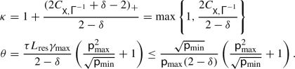
Theorem 4.2

Let $(\varvec{x}^k)_{k \in \mathbb {N}}$ be generated by Algorithm 1.1 and suppose $\delta <2$ and that the error bound condition (4.1) holds with ${\textsf{X}}\supset \{\varvec{x}^k\,\vert \,k \in \mathbb {N}\}$ ${\textsf{P}}$-a.s. for some . Then for all $k \in \mathbb {N}$,

• (i) $\displaystyle {\textsf{E}}\big [F(\varvec{x}^{k+1})-F^*\big ] \le \left( 1 - \frac{\textsf{p}_{\min }}{\kappa +\theta }\right) ^{\lfloor \frac{k+1}{\tau + 1} \rfloor } {\textsf{E}}\big [F(\varvec{x}^{0})-F^*\big ],$

  where

  

• (ii) The sequence $(\varvec{x}^k)_{k\in \mathbb {N}}$ converges strongly ${\textsf{P}}$-a.s. to a random variable $\varvec{x}^*$ that takes values in ${{\,\mathrm{\mathrm {{argmin}}}\,}}F$ and .

Proof

(i): From Proposition 3.6 we have

where $\alpha _k = (L_{\textrm{res}}/(2\sqrt{\textsf{p}_{\min }})) \sum _{h = k-\tau }^{k-1} (h-(k-\tau )+1)\Vert \varvec{x}^{h+1} - \varvec{x}^{h}\Vert _{{\textsf{V}}}^2$. Now, taking $\varvec{{\textsf{x}}}\in {{\,\mathrm{\mathrm {{argmin}}}\,}}F$ and using the error bound condition (4.1) and Eq. (3.3), we obtain

(4.2)

Adding and removing $F^*$ in both expectation yield

(4.3)

where . Now, since $\Vert \cdot \Vert ^2_{{\textsf{V}}} \le \gamma _{\max }\textsf{p}_{\max }^2 \Vert \cdot \Vert ^2_{{\textsf{W}}}$ we have

(4.4)

where in the last equality we used Lemma 3.5. From (3.3), we have, for k such that $k-\tau \ge 0$,

(4.5)

Since the sequence $\left( {\textsf{E}}\big [F(\varvec{x}^{k})+\alpha _{k}\big ]\right) _{k \in \mathbb {N}}$ is decreasing, the transition from the second line to the third one is allowed. Using (4.4) and (4.5) in (4.3) with total expectation and recalling the definition of $\theta$, we obtain

$$\begin{aligned} (\kappa +\theta ){\textsf{E}}\big [F(\varvec{x}^{k+1})+\alpha _{k+1}-F^*\big ]&\le (\kappa - \textsf{p}_{\min }) {\textsf{E}}\big [F(\varvec{x}^{k})+\alpha _{k}-F^*\big ] \nonumber \\&\qquad + \theta {\textsf{E}}\big [F(\varvec{x}^{k - \tau })+\alpha _{k-\tau }-F^*\big ] \nonumber \\&\le (\kappa - \textsf{p}_{\min }) {\textsf{E}}\big [F(\varvec{x}^{k-\tau })+\alpha _{k-\tau }-F^*\big ] \nonumber \\&\qquad + \theta {\textsf{E}}\big [F(\varvec{x}^{k - \tau })+\alpha _{k-\tau }-F^*\big ] \nonumber \\&= (\kappa + \theta - \textsf{p}_{\min }) {\textsf{E}}\big [F(\varvec{x}^{k-\tau })+\alpha _{k-\tau }-F^*\big ]. \end{aligned}$$

(4.6)

That means

$$\begin{aligned} {\textsf{E}}\big [F(\varvec{x}^{k+1})+\alpha _{k+1}-F^*\big ]&\le \left( 1 - \frac{\textsf{p}_{\min }}{\kappa +\theta }\right) {\textsf{E}}\big [F(\varvec{x}^{k-\tau })+\alpha _{k-\tau }-F^*\big ] \nonumber \\&\le \left( 1 - \frac{\textsf{p}_{\min }}{\kappa +\theta }\right) ^{\lfloor \frac{k+1}{\tau + 1} \rfloor } {\textsf{E}}\big [F(\varvec{x}^{0})+\alpha _{0}-F^*\big ]. \end{aligned}$$

(4.7)

Now for $k < \tau$, $\lfloor \frac{k+1}{\tau + 1} \rfloor = 0$. Since $\left( {\textsf{E}}\big [F(\varvec{x}^{k}) +\alpha _{k}\big ]\right) _{k \in \mathbb {N}}$ is decreasing, we know that

$$\begin{aligned} {\textsf{E}}\big [F(\varvec{x}^{k+1})+\alpha _{k+1}-F^*\big ]&\le {\textsf{E}}\big [F(\varvec{x}^{0})+\alpha _{0}-F^*\big ] \\&= \left( 1 - \frac{\textsf{p}_{\min }}{\kappa +\theta }\right) ^{\lfloor \frac{k+1}{\tau + 1} \rfloor } {\textsf{E}}\big [F(\varvec{x}^{0})+\alpha _{0}-F^*\big ]. \end{aligned}$$

So (4.7) remains true. Also from (B.10), we have

$$\begin{aligned} \theta \le \frac{\sqrt{\textsf{p}_{\min }}}{\textsf{p}_{\max }}(2-\delta )^{-1} \left( \frac{\textsf{p}^2_{\max }}{\sqrt{\textsf{p}_{\min }}} + 1 \right) . \end{aligned}$$

(ii): From Jensen inequality, (3.3) and (4.7), we have

(4.8)

Since $1 - \textsf{p}_{\min }/(\kappa +\theta ) < 1$,

Therefore ${\textsf{P}}$-a.s. This means that the sequence $(\varvec{x}^k)_{k\in \mathbb {N}}$ is a Cauchy sequence ${\textsf{P}}$-a.s. By Theorem 3.1(i), this sequence converges weakly $\textsf {P}$-a.s. to a random variable which takes values in ${{\,\mathrm{\mathrm {{argmin}}}\,}}F$. So it converges strongly ${\textsf{P}}$-a.s. to that the same random variable taking values in ${{\,\mathrm{\mathrm {{argmin}}}\,}}F$.

Now let $\rho = 1 - \textsf{p}_{\min }/(\kappa +\theta )$. For all $n \in \mathbb {N}$,

Letting $n \rightarrow \infty$ and using (4.8), we get

$\square$

Remark 4.3

• (i) A linear convergence rate is also given in [31, Theorem 4.1] by assuming a quadratic growth condition instead of the error bound condition (4.1). Their rate depend on the stepsize which in general can be very small, as explained earlier in point (vi) of Remark 3.2.

• (ii) The error bound condition (4.1) is sometimes satisfied globally, meaning on ${\textsf{X}}= {{\,\mathrm{\text {{dom}}}\,}}F$, so that the condition ${\textsf{X}}\supset \{\varvec{x}^k\,\vert \,k \in \mathbb {N}\}$ ${\textsf{P}}$-a.s. required in Theorem 4.2 is clearly fulfilled. This is the case when F is strongly convex or when f is quadratic and g is the indicator function of a polytope (see Remark 4.17(iv) in [42]). More often, for general convex objectives, the error bound condition (4.1) is satisfied on sublevel sets of F (see [42, Remark 4.18]). Therefore, it is important to find conditions ensuring that the sequence $(\varvec{x}^k)_{k \in \mathbb {N}}$ remains in a sublevel set. The next results address this issue.

We first give an analogue of Lemma 3.4.

Lemma 4.4

Let $(\varvec{x}^k)_{k \in \mathbb {N}}$ be the sequence generated by Algorithm 1.1. Then, for every $k \in \mathbb {N}$,

$$\begin{aligned} \langle \nabla f(\varvec{x}^k) - \nabla f({\hat{\varvec{x}}}^k), {x}^{k+1} - x^k\rangle \le \tau L_{\textrm{res}} \Vert {\varvec{x}}^{k+1} - \varvec{x}^k\Vert ^2 + {\tilde{\alpha }}_k - {\tilde{\alpha }}_{k+1}, \end{aligned}$$

with ${\tilde{\alpha }}_k = (L_{\textrm{res}}/2)\sum _{h = k-\tau }^{k-1} (h-(k-\tau )+1)\Vert \varvec{x}^{h+1} - \varvec{x}^{h}\Vert ^2$.

Proof

Let $k \in \mathbb {N}$. We have, from Cauchy-Schwarz inequality, the Young inequality, and Lemma 2.5, that

$$\begin{aligned} \langle \nabla f(\varvec{x}^k)&-\nabla f({\hat{\varvec{x}}}^k),{\varvec{x}}^{k+1}-\varvec{x}^k \rangle \\&\le L_{\textrm{res}} \sum _{h \in J(k)} \Vert \varvec{x}^{h+1} - \varvec{x}^{h}\Vert \Vert {\varvec{x}}^{k+1} - \varvec{x}^k\Vert \\&\le \frac{1}{2}\left[ \frac{L_{\textrm{res}}^2}{s}\bigg (\sum _{h \in J(k)} \Vert \varvec{x}^{h+1} - \varvec{x}^{h}\Vert \bigg )^2 +s\Vert {\varvec{x}}^{k+1} - \varvec{x}^k\Vert ^2\right] \\&\le \frac{1}{2}\left[ \frac{\tau L_{\textrm{res}}^2}{s}\left( \sum _{h = k-\tau }^{k-1} \Vert \varvec{x}^{h+1} - \varvec{x}^{h}\Vert ^2\right) +s\Vert {\varvec{x}}^{k+1} - \varvec{x}^k\Vert ^2\right] \\&= \frac{s}{2}\Vert {\varvec{x}}^{k+1} - \varvec{x}^k\Vert ^2 + \frac{\tau L_{\textrm{res}}^2}{2s}\sum _{h = k-\tau }^{k-1} \Vert \varvec{x}^{h+1} - \varvec{x}^{h}\Vert ^2. \end{aligned}$$

Using the same decomposition of the last term as in Lemma 3.4, we get

$$\begin{aligned} \langle \nabla f(\varvec{x}^k)&- \nabla f({\hat{\varvec{x}}}^k), {\varvec{x}}^{k+1} - \varvec{x}^k\rangle \\&\le \frac{s}{2}\Vert {\varvec{x}}^{k+1} - \varvec{x}^k\Vert ^2 + \frac{\tau L_{\textrm{res}}^2}{2s} \sum _{h = k-\tau }^{k-1} (h- (k-\tau )+1)\Vert \varvec{x}^{h+1} - \varvec{x}^{h}\Vert ^2 \\&\qquad - \frac{\tau L_{\textrm{res}}^2}{2s} \sum _{h=k-\tau +1}^{k} (h-(k-\tau ))\Vert \varvec{x}^{h+1} - \varvec{x}^{h}\Vert ^2 \\&\qquad + \frac{\tau ^2 L_{\textrm{res}}^2}{2s} \Vert \varvec{x}^{k+1} - \varvec{x}^{k}\Vert ^2. \end{aligned}$$

So taking

$$\begin{aligned} \displaystyle {\tilde{\alpha }}_k = \frac{\tau L_{\textrm{res}}^2}{2s}\sum _{h = k-\tau }^{k-1} (h-(k-\tau )+1)\Vert \varvec{x}^{h+1} - \varvec{x}^{h}\Vert ^2, \end{aligned}$$

we get

$$\begin{aligned} \langle \nabla f(\varvec{x}^k) - \nabla f({\hat{\varvec{x}}}^k), {\bar{x}}^{k+1} - x^k\rangle \le \left( \frac{s}{2} + \frac{\tau ^2 L_{\textrm{res}}^2}{2s} \right) \Vert {\bar{\varvec{x}}}^{k+1} - \varvec{x}^k\Vert ^2 + {\tilde{\alpha }}_k - {\tilde{\alpha }}_{k+1}. \end{aligned}$$

By minimizing $s \mapsto (s/2 + \tau ^2 L_{\textrm{res}}^2/(2s))$, we find $s=\tau L_{\textrm{res}}$. We then obtain

$$\begin{aligned} \langle \nabla f(\varvec{x}^k) - \nabla f({\hat{\varvec{x}}}^k), {x}^{k+1} - x^k\rangle \le \tau L_{\textrm{res}} \Vert {\varvec{x}}^{k+1} - \varvec{x}^k\Vert ^2 + {\tilde{\alpha }}_k - {\tilde{\alpha }}_{k+1}, \end{aligned}$$

and the statement follows. $\square$

Proposition 4.5

Let $(\varvec{x}^k)_{k \in \mathbb {N}}$ be the sequence generated by Algorithm 1.1. Then, for every $k \in \mathbb {N}$,

$$\begin{aligned} \bigg (\frac{1}{\gamma _{i_{k}}}-\frac{L_{i_{k}}}{2} -\tau L_{\textrm{res}}\bigg )\Vert \varvec{x}^{k+1} - \varvec{x}^k\Vert ^2 \le F(\varvec{x}^k)+ {\tilde{\alpha }}_k - \big (F(\varvec{x}^{k+1}) +{\tilde{\alpha }}_{k+1} \big ) \qquad {\textsf{P}}\text {-a.s.},\nonumber \\ \end{aligned}$$

(4.9)

where ${\tilde{\alpha }}_k = (L_{\textrm{res}}/2)\sum _{h = k-\tau }^{k-1} (h-(k-\tau )+1)\Vert \varvec{x}^{h+1} - \varvec{x}^{h}\Vert ^2$.

Proof

Using Lemma 4.4 in Eq. (B.3), we have

$$\begin{aligned} F(\varvec{x}^{k+1})&\le F(\varvec{x}^k) + \langle \nabla _{i_{k}} f(\varvec{x}^k) - \nabla _{i_{k}} f({\hat{\varvec{x}}}^k), {\bar{x}}^{k+1}_{i_{k}} - x^k_{i_{k}} \rangle - \bigg (\frac{1}{\gamma _{i_{k}}}-\frac{L_{i_{k}}}{2}\bigg )|{\bar{x}}^{k+1}_{i_{k}} - x^k_{i_{k}}|^2 \\&= F(\varvec{x}^k) + \langle \nabla f(\varvec{x}^k) - \nabla f({\hat{\varvec{x}}}^k), \varvec{x}^{k+1} - \varvec{x}^k \rangle - \bigg (\frac{1}{\gamma _{i_{k}}}-\frac{L_{i_{k}}}{2}\bigg )\Vert \varvec{x}^{k+1} - \varvec{x}^k\Vert ^2 \\&\le F(\varvec{x}^k) + {\tilde{\alpha }}_k - {\tilde{\alpha }}_{k+1} - \bigg (\frac{1}{\gamma _{i_{k}}}-\frac{L_{i_{k}}}{2} - \tau L_{\textrm{res}}\bigg )\Vert \varvec{x}^{k+1} - \varvec{x}^k\Vert ^2. \end{aligned}$$

So the statement follows. $\square$

Corollary 4.6

Let $(\varvec{x}^k)_{k \in \mathbb {N}}$ be generated by Algorithm 1.1 with the $\gamma _i$’s satisfying the following stepsize rule

$$\begin{aligned} (\forall \, i \in [m])\quad \gamma _i < \frac{2}{L_{i} + 2\tau L_{\textrm{res}}}. \end{aligned}$$

(4.10)

Then

$$\begin{aligned} (\forall \, k \in \mathbb {N})\quad F(\varvec{x}^k) \le F(\varvec{\textsf{x}}^0) \quad {\textsf{P}}\text {-a.s.} \end{aligned}$$

(4.11)

So if the error bound condition (4.1) holds on the sublevel set ${\textsf{X}}= \{F \le F(\varvec{\textsf{x}}^0)\}$, then the assumptions of Theorem 4.2 are met.

Proof

The left hand side in (4.9) is positive and hence $(F(\varvec{x}_k) + {\tilde{\alpha }}_k)_{k \in \mathbb {N}}$ is decreasing ${\textsf{P}}$-a.s. Therefore, we have, for every $k \in \mathbb {N}$

$$\begin{aligned} F(\varvec{x}^{k}) \le F(\varvec{x}^{k}) +{\tilde{\alpha }}_{k} \le F(\varvec{x}^0) + {\tilde{\alpha }}_0 = F(\varvec{\textsf{x}}^0). \end{aligned}$$

Remark 4.7

The rule (4.10) yields stepsizes possibly smaller than the ones given in Theorem 3.1, which requires $\gamma _i< 2/(L_{i} + 2\tau L_{\textrm{res}}\textsf{p}_{\max }/\sqrt{\textsf{p}_{\min }})$. Indeed this happens when $\textsf{p}_{\max }/\sqrt{\textsf{p}_{\min }} < 1$. For instance if the distribution is uniform, we have $\textsf{p}_{\max }/\sqrt{\textsf{p}_{\min }} = 1/\sqrt{m} < 1$ whenever $m \ge 2$. On the bright side, there may exist distributions for which $\textsf{p}_{\max }/\sqrt{\textsf{p}_{\min }} > 1$.

5 Applications

Here we present two problems where Algorithm 1.1 can be useful.

5.1 The Lasso problem

We start with the Lasso problem [47], also known as basis pursuit [11]. It is a least-squares regression problem with an $\ell _1$ regularizer which favors sparse solutions. More precisely, given ${\textsf{A}}\in \mathbb {R}^{n \times m}$ and $\textsf{b}\in \mathbb {R}^n$, one aims at solving the following problem

$$\begin{aligned} \underset{\varvec{\textsf{x}}\in \mathbb {R}^m}{\text {minimize }} \frac{1}{2}\Vert {\textsf{A}}\varvec{\textsf{x}}- \textsf{b}\Vert _2^2 + \lambda \Vert \varvec{\textsf{x}}\Vert _1 \qquad \left( \lambda > 0\right) . \end{aligned}$$

(5.1)

We clearly fall in the framework of problem (1.1) with $f(\varvec{\textsf{x}}) = (1/2)\Vert {\textsf{A}}\varvec{\textsf{x}}- \textsf{b}\Vert _2^2$ and $g_i(\textsf{x}_i) = \lambda |\textsf{x}_i|$. The assumptions A1, A2, A3 and A4 are also satisfied. In particular, here $L_i = \Vert A_{.i}\Vert ^2$, where $A_{.i}$ is the i-th column of ${\textsf{A}}$, $L_{\textrm{res}} = \max _{i}\Vert ({\textsf{A}}^{\intercal }{\textsf{A}})_{\cdot i}\Vert _{2}$, with $({\textsf{A}}^{\intercal }{\textsf{A}})_{\cdot i}$ the i-th column of ${\textsf{A}}^{\intercal }{\textsf{A}}$, and $F = f + g$ attains its minimum.

The Lasso technique is used in many fields, especially for high-dimensional problems – among others it is worth mentioning statistics, signal processing, and inverse problems; see [4, 5, 17, 25, 46, 48] and references therein. Since there is no closed form solution for this problem, many iterative algorithms have been proposed to solve it: forward-backward, accelerated (proximal) gradient descent, (proximal) block coordinate descent, etc. [4, 15, 21, 22, 38, 49]. In the same vein, applying Algorithm 1.1 to the Lasso problem (5.1) yields the iterative scheme:

$$\begin{aligned} \begin{array}{l} \text {for}\;n=0,1,\ldots \\ \left\lfloor \begin{array}{l} \text {for}\;i=1,\dots , m\\ \left\lfloor \begin{array}{l} x^{k+1}_i = {\left\{ \begin{array}{ll} {\textsf{soft}}_{\lambda \gamma _{i_{k}}} \big (x^k_{i_{k}} - \gamma _{i_{k}} a_{i_k}^\intercal ( {\textsf{A}}\varvec{x}^{k-\varvec{{\textsf{d}}}^k} - \textsf{b}) \big ) &{}\text {if } i=i_{k}\\ x^k_i &{}\text {if } i \ne i_{k}, \end{array}\right. } \end{array} \right. \end{array} \right. \end{array} \end{aligned}$$

(5.2)

where, for every $\rho >0$, $\textsf{soft}_{\rho }:\mathbb {R}\rightarrow \mathbb {R}$ is the soft thresholding operator (with threshold $\rho$) [43]. Thanks to Theorem 3.1 we know that the iterates $(\varvec{x}^k)_{k \in \mathbb {N}}$ generated are weakly convergent and the function values have a convergence rate of o(1/k). On top of that the cost function of the Lasso problem (5.1) satisfies the error bound condition (4.1) on its sublevel sets [50, Theorem 2]. So, following Corollary 4.6 and Theorem 4.2, the iterates converge strongly (a.s.) and linearly in mean, whenever $\gamma _i < 2/\left( L_{i} + 2\tau L_{\textrm{res}}\right)$, for all $i \in [m]$.

5.2 Linear convergence of dual proximal gradient method

We consider the problem

$$\begin{aligned} \underset{\textsf{x}\in \textsf{H}}{\text {minimize }}\sum _{i=1}^{m} \phi _{i}\left( {\textsf{A}}_i\textsf{x}\right) + h(\textsf{x}), \end{aligned}$$

(5.3)

where, for all $i \in [m], {\textsf{A}}_i:\textsf{H}\rightarrow \textsf{G}_i$ is a linear operator between Hilbert spaces, $\phi _{i}:\textsf{G}_i \rightarrow ]-\infty ,+\infty ]$ is proper convex and lower semicontinuous, and $h:\textsf{H}\rightarrow ]-\infty ,+\infty ]$ is proper lower semicontinuous and $\sigma$-strongly convex $(\sigma >0)$. The first term of the objective function may represent the empirical data loss and the second term the regularizer. This problem arises in many applications in machine learning, signal processing and statistical estimation, and is commonly called regularized empirical risk minimization [44]. It includes, for instance, ridge regression and (soft margin) support vector machines [44], more generally Tikhonov regularization [26, Section 5.3].

In the following we apply Algorithm 1.1 to the dual of problem (5.3). Below we provide details. Set $\varvec{\textsf{G}}=\bigoplus _{i=1}^m \textsf{G}_i$ and $\varvec{\textsf{u}}= (\textsf{u}_{1}, \textsf{u}_{2}, \ldots , \textsf{u}_{m})$. Then, the dual of problem (5.3) is

$$\begin{aligned} \underset{\varvec{\textsf{u}}\in \mathbf {\textsf{G}}}{\text {minimize }} F(\varvec{\textsf{u}}) = h^*\bigg (-\sum _{i=1}^{m} {\textsf{A}}^*_i\textsf{u}_{i}\bigg ) + \sum _{i=1}^m \phi ^*_i(\textsf{u}_i), \end{aligned}$$

(5.4)

where, ${\textsf{A}}_i^*$ is the adjoint operator of ${\textsf{A}}_i$ $h^*$ and $\phi _i^*$ are the Fenchel conjugates of h and $\phi _i$ respectively. The link between the dual variable $\varvec{\textsf{u}}$ and the primal variable $\textsf{x}$ is given by the rule $\varvec{\textsf{u}}\mapsto \nabla h^*(-\sum _{i=1}^{m} {\textsf{A}}^*_i\textsf{u}_{i})$. Since $h^*$ is $(1/\sigma )$-Lipschitz smooth, the dual problem above is in the form of problem (1.1). Thus, Algorithm (1.1) applied to the dual problem (5.4) gives

$$\begin{aligned} \begin{array}{l} \text {for}\;k=0,1,\ldots \\ \left\lfloor \begin{array}{l} \text {for}\;i=1,\dots , m\\ \left\lfloor \begin{array}{l} u^{k+1}_i = {\left\{ \begin{array}{ll} {\textsf {prox}}_{\gamma _{i_{k}} \phi _{i_{k}}^*}\big (u_{i_{k}}^{k}+\gamma _{i_{k}} {\textsf{A}}_{i_k}\nabla h^{*}( - \sum _{j=1}^{m} {\textsf{A}}^*_j u^{k - \textsf{d}^k_j}_{j}) \big ) &{}\text {if } i=i_{k}\\ u^k_i &{}\text {if } i \ne i_{k}, \end{array}\right. } \end{array} \right. \end{array} \right. \end{array} \end{aligned}$$

(5.5)

Suppose that $\nabla h^{*} = {\textsf{B}}$ is a linear operator and that the delay vector $\varvec{{\textsf{d}}}^k= (\textsf{d}_1^k,\ldots , \textsf{d}_m^k)$ is uniform, that is, $\textsf{d}^k_i = \textsf{d}^k \in \mathbb {N}$. Then, using the primal variable, the KKT condition $x^k = \nabla h^{*}( -\sum _{j=1}^{m} {\textsf{A}}^*_j u^{k}_{j}) = - \sum _{j=1}^{m} {\textsf{B}}{\textsf{A}}^*_j u^{k}_{j}$, and the fact that $\varvec{u}^{k+1}$ and $\varvec{u}^k$ differ only on the $i_k$-component, the algorithm becomes

$$\begin{aligned} \begin{array}{l} \text {for}\;k=0,1,\ldots \\ \left\lfloor \begin{array}{l} \text {for}\;i=1,\dots , m\\ \left\lfloor \begin{array}{l} u^{k+1}_i = {\left\{ \begin{array}{ll} {\textsf {prox}}_{\gamma _{i_{k}} \phi _{i_{k}}^*}\big (u_{i_{k}}^{k}+\gamma _{i_{k}} {\textsf{A}}_{i_k} \varvec{x}^{k-\textsf{d}^k}\big ) &{}\text {if } i=i_{k}\\ u^k_i &{}\text {if } i \ne i_{k}. \end{array}\right. }\\ \text { }\\ \varvec{x}^{k+1} = \varvec{x}^k - {\textsf{B}}{\textsf{A}}^*_{i_k} (u^{k+1}_{i_k} - u^{k}_{i_k}). \end{array} \right. \end{array} \right. \end{array} \end{aligned}$$

(5.6)

The above algorithm requires a lock during the update of the primal variable $\textsf{x}$. On the contrary, the update of the dual variable $\varvec{\textsf{u}}$ is completely asynchronous without any lock as in the setting we studied in this paper. To get a better understanding of this aspect, we will expose a concrete example: the ridge regression.

5.2.1 Example: ridge regression

The ridge regression is the following regularized least squares problem.

$$\begin{aligned} \underset{\textsf{w}\in \textsf{H}}{\text {minimize}}\, \frac{1}{\lambda m} \sum _{i=1}^{m} \left( \textsf{y}_{i} - \left\langle \textsf{w}, \textsf{x}_{i}\right\rangle \right) ^2 +\frac{1}{2}\Vert \textsf{w}\Vert ^{2}. \end{aligned}$$

(5.7)

Its dual problem is

$$\begin{aligned} \underset{\varvec{\textsf{u}}\in \mathbb {R}^m}{\text {minimize}}\, \frac{1}{2} \langle (\textsf{K}+\lambda m \textsf{Id}_m) \varvec{\textsf{u}}, \varvec{\textsf{u}}\rangle -\langle \varvec{\textsf{y}},\varvec{\textsf{u}}\rangle , \end{aligned}$$

where $\textsf{K}= \textsf{X}\textsf{X}^{*}$ and $\textsf{X}:\textsf{H}\rightarrow \mathbb {R}^m$, with $\textsf{X}\textsf{w}= (\langle \textsf{w},\textsf{x}_i\rangle )_{1 \le i\le m}$. We remark that, in this situation, $A_i = \langle \cdot , \textsf{x}_i\rangle$, $A_i^* = \textsf{x}_i$ and $B=\textsf{Id}$. Let $\varvec{{\textsf{d}}}^k= (\textsf{d}^k, \textsf{d}^k, \ldots , \textsf{d}^k)$. With $\textsf{w}^k = \textsf{X}^{*}\varvec{\textsf{u}}^k$ and considering that the non smooth part g is null, the algorithm is given by

$$\begin{aligned} \begin{array}{l} \text {for}\;k=0,1,\ldots \\ \left\lfloor \begin{array}{l} \text {for}\;i=1,\dots , m\\ \left\lfloor \begin{array}{l} u^{k+1}_i = {\left\{ \begin{array}{ll} u_{i_{k}}^{k} - \gamma _{i_{k}} \big (\langle \textsf{x}_{i_k}, \varvec{w}^{k-\textsf{d}^k}\rangle +\lambda m u_{i_k}^{k-\textsf{d}^{k}}-\textsf{y}_{i_k}\big ) &{}\text {if } i=i_{k}\\ u^k_i &{}\text {if } i \ne i_{k}. \end{array}\right. }\\ \text { }\\ \varvec{w}^{k+1} = \varvec{w}^k - \gamma _{i_{k}} \textsf{x}_{i_k}\big (\textsf{u}^{k+1}_{i_k} - \textsf{u}^k_{i_k}\big ). \end{array} \right. \end{array} \right. \end{array} \end{aligned}$$

(5.8)

Remark 5.1

Now we will compare the above dual asynchronous algorithm to the asynchronous stochastic gradient descent (ASGD) [1, 39]. We note that (5.8) yields

$$\begin{aligned} \varvec{w}^{k+1}&= \varvec{w}^k - \gamma _{i_{k}} \textsf{x}_{i_k}\big (u^{k+1}_{i_k} - u^k_{i_k}\big ) \\&= \varvec{w}^k - \gamma _{i_{k}} \big (\langle \textsf{x}_{i_k}, \varvec{w}^{k-\textsf{d}^k}\rangle \textsf{x}_{i_k} +\lambda m u_{i_k}^{k-\textsf{d}^k}\textsf{x}_{i_k} -\textsf{y}_{i_k}\textsf{x}_{i_k}\big ). \end{aligned}$$

Instead, applying asynchronous SGD to the primal problem (5.7) multiply by $\lambda m$, we get

$$\begin{aligned} \varvec{w}^{k+1} = \varvec{w}^k - \gamma _{k}^{\prime } \big (\langle \textsf{x}_{i_k}, \varvec{w}^{k-\textsf{d}^k}\rangle \textsf{x}_{i_k} +\lambda m \varvec{w}^{k-\textsf{d}^k}-\textsf{y}_{i_k}\textsf{x}_{i_k}\big ). \end{aligned}$$

We see that the only difference is the second term inside the parentheses in both updates. Indeed the term $\varvec{w}^{k-\textsf{d}^k} = \textsf{X}^{*}\varvec{u}^{k-\textsf{d}^k} = \sum _{i=1}^m u_{i}^{k-\textsf{d}^k}\textsf{x}_{i}$ in ASGD is replaced by only one summand $u_{i_k}^{k-\textsf{d}^k}\textsf{x}_{i_k}$ in our algorithm. However, a major difference between the two approaches lies in the way the stepsize is set. Indeed, in ASGD, the stepsize $\gamma _k^{\prime }$ is chosen with respect to the operator norm of $\textsf{K}+ \lambda m \textsf{Id}$ i.e., the Lipschitz constant of the full gradient of the primal objective function, see [1, Theorem 1]. By contrast, in algorithm (5.8), for all $i \in [m]$, the stepsizes $\gamma _i^k$ are chosen with respect to the Lipschitz constant of the partial derivatives of the dual objective function i.e., $\textsf{K}_{i,i} + \lambda m$. Not only the latter are easier to compute, they also allow for possibly longer steps along the coordinates.

6 Experiments

In this section, we will present some experiments with the purpose of assessing our theoretical findings and making comparison with related results in the literature. All the codes are available on GitHub.¹

We coded the mathematical model of asynchronicity in (1.2). At each iteration we compute the forward step using gradients that are possibly outdated. The delay vector components are a priori chosen according to a uniform distribution on $\{0,1,\ldots ,\tau \}$. The block coordinates are updated with a uniform distribution independent from the delay vector. We considered three kinds of experiments: in the first one we did a speedup test for our algorithm on the Lasso problem. This allows to check whether the speed of convergence increases linearly with the number of machines used. Then, we considered a comparison with the synchronous version of the algorithm in order to show the advantage of the asynchronous implementation. Finally, in the third group of experiments we compared our algorithm with those by Liu et al. [31] and Cannelli et al. [8].

6.1 Speedup test

In this section we consider the Lasso problem (5.1) with $n=100$ and $m \in \{500, 1000, 2000, 8000\}$. The parameter $\lambda$ is chosen small enough so that the minimizer $\varvec{x}^*$ has non zero components. For more flexibility, we used synthetic data, which were generated using the function make_correlated_data of the Python library celer. This function creates a matrix ${\textsf{A}}$ with columns generated according to the Autoregressive (AR) model.² Then $\textsf{b}$ is generated as $\textsf{b}= {\textsf{A}}\varvec{w}+ \epsilon$, where $\epsilon$ is a Gaussian random vector, with zero mean and variance equal to the identity, such that the signal to noise ration (SNR) is 3 and $\varvec{w}$ is a vector with $1\%$ of nonzero entries. The nonzero blocks of $\varvec{w}$ are chosen uniformly and their entries are generated according to the standard normal distribution. As in [8, 31], we make the assumption that $\tau$ is proportional to the number of machines. Since we use 10 cores, we fix $\tau = 10$ like in [28]. For a fixed data, we run the algorithm 10 times and average it. Similarly to [8, 31], in our experiment the speedup gets better when we increase the number of blocks, see Fig. 1. This can be explained by the fact that the algorithm has to run long enough in order to minimize the cost of parallelization—the initialization cost, the mandatory locks in order to avoid data racing, etc. Also, if there are more blocks, the probability of two machines having to write on the same block at the same time is reduced and so is the number of locks. All these observations align with the known fact that the more there are cores, the more the problem should be complex to see good speedup.

Fig. 1

The plots showed the speedup obtain by Algorithm 1.1 compared to the ideal speedup for different number of blocks. The shaded zones illustrate the standard deviation of the results over 10 trials

Fig. 2

Comparison of Algorithm 1.1 to its synchronous counterpart

6.2 Comparison with the synchronous version

We compared Algorithm 1.1 to its synchronous counterpart in the Lasso case. The data, as well as the parameters, is generated as in the speedup experiment. The step size of the synchronous algorithm is set as suggested in [42] for a non sparse matrix ${\textsf{A}}$. We run both algorithms for 120 seconds and compare the distances of their function values to the minimum. As expected, Algorithm 1.1 is faster; see Fig. 2.

6.3 Comparison with other asynchronous algorithms

In this section we illustrate the results of the comparison with the algorithms proposed in [31] and [8]. As for [8], we set (in the notation of the paper) the relaxation parameter $\gamma = 1$ and $c_{\tilde{f}}=2\beta$ so that

$$\begin{aligned} x^{k+1}_i = {\left\{ \begin{array}{ll} {\textsf {prox}}_{ (1/2\beta ) g_{i}} \big (x^{k-d^k_{i}}_{i} - (1/2\beta ) \nabla _{i} f (\varvec{x}^{k-\varvec{{\textsf{d}}}^k})\big ) &{}\text {if } i=i_{k}\\ x^k_i &{}\text {if } i \ne i_{k}. \end{array}\right. } \end{aligned}$$

Then, according to Theorem 1 in [8], we choose $2\beta > L_f(1+\delta ^2/2)$ where $\delta = \tau$ is the maximum delay. We note that this model is slightly different from ours since the delay is present not only in the gradient.

In [31], the same algorithm as (1.2) is considered, but with a stepsize $\gamma$ which is the same for all the blocks. In our comparisons, we choose the step according to the conditions required by the main Theorem 4.1 in [31], since the hypotheses of Corollary 4.2 are not satisfied for our datasets³, see the discussion in Remark 3.2 (vi). If $\tau$ is the maximum delay, Theorem 4.1 in [31] requires the following conditions on the stepsize:

$$\begin{aligned} \gamma < \frac{\sqrt{n}(1-\rho ^{-1})-4}{4(1+\theta )L_{\text {res}}/L'_{\max }} \quad \text {with}\ \theta =\frac{\rho ^{(\tau +1) / 2}-\rho ^{1 / 2}}{\rho ^{1 / 2}-1}, \end{aligned}$$

which only make sense if the right hand side is strictly positive, so when $n > 16$ and $\rho > \frac{1 + 4/\sqrt{n}}{1 - 16/n}$ (instead of $\rho > 1 + 4/\sqrt{n}$ as claimed in [31]). So, in the experiments, we set $\rho > \frac{1 + 4/\sqrt{n}}{1 - 16/n}$. This leads in general to very small stepsizes, as we will further discuss in the next section.

Fig. 3

The plots show the behavior of $F(\varvec{x}_k)- F^*$ for the 3 algorithms applied to a lasso loss with different values of $\tau$: 5, 10, 15, 20

6.3.1 Lasso problem

In this section we consider the Lasso problem (5.1) with $m=90$, $n=51630$, and $\lambda =0.01$. We use the data YearPredictionMSD.t from libsvm⁴ to generate the matrix ${\textsf{A}}$. Before showing the results, we briefly comment on the experimental set-up. As shown in Sect. 5.1, in this case $L_i=\Vert {\textsf{A}}_{\cdot i}\Vert _2^2$ and $L_{\textrm{res}}=\max _{i}\Vert ({\textsf{A}}^{\intercal }{\textsf{A}})_{\cdot i}\Vert _{2}$. In [8], $L_f=L_{\textrm{res}}$ and in [31] $L'_{\max }=\max _{i}\Vert ({\textsf{A}}^{\intercal }{\textsf{A}})_{\cdot i}\Vert _{\infty }$.

Looking at the results, we see that our algorithm outperforms those in [31] and [8], see Fig. 3. This difference is due to the fact that our stepsize is bigger than the other two. Indeed, in [31] and [8] the stepsizes have a worse dependence on the maximum delay $\tau$ (inverse quadratically in [8] and exponentially in [31]), which ultimately shorten the stepsizes. Also, in both [31] and [8] the stepsize is the same for all the blocks, so the algorithm is more sensitive to the conditioning of the problem. An overall comparison of the effect of $\tau$ on the stepsize is shown in Fig. 4.

Fig. 4

This figure shows how the minimum of our stepsizes fares against the two others when $\tau$ increases on a lasso problem

6.3.2 Logistic regression

For another comparison, next we consider the $\ell _1$ regularized logistic loss:

$$\begin{aligned} F(x) = \frac{1}{n} \sum _{i=1}^n \log (1+\exp \{-b_i\langle a_i, \varvec{x}\rangle \}) + \lambda \Vert \varvec{x}\Vert _{1}. \end{aligned}$$

(6.1)

For this experiment we use the data Splice.t from libsvm⁵ with $m=60$, $n=2175$, and $\lambda =0.01$. Let ${\textsf{A}}\in \mathbb {R}^{m \times n}$ be the matrix with columns the $a_i$’s ($i \in [n]$). We denote by $\Vert \cdot \Vert$, $\Vert \cdot \Vert _{\infty }$, $\Vert \cdot \Vert _{F}$, the spectral norm, the infinity norm, and the Frobenius norm of matrices, respectively. The relevant constants for the stepsizes are

• $L_{\textrm{res}}= \frac{1}{n}\Vert {\textsf{A}}\Vert \max _j \Vert {\textsf{A}}_{j \cdot }\Vert _2$ for our algorithm and [31],

• $L^\prime _{\max } = \frac{1}{n} \Vert {\textsf{A}}\Vert _{\infty } \max _j \Vert {\textsf{A}}_{j \cdot }\Vert _{\infty }$ for [31],

• $L_j = \frac{1}{n}\Vert {\textsf{A}}_{j \cdot }\Vert _2^2$, $j \in [m]$, for our algorithm, where ${\textsf{A}}_{j \cdot }$ is the j-th row of ${\textsf{A}}$.

• $L_f = \frac{1}{n}\Vert {\textsf{A}}\Vert _{F} \max _j \Vert {\textsf{A}}_{j \cdot }\Vert _2$ for [8].

So, the stepsizes range from about $1.1191*10^{-3} \text { to } 7.5164*10^{-3}$ for [8], $5.6537*10^{-8} \text { to } 2.1571*10^{-10}$ for [31], and $2.2605*10^{-2} \text { to } 6.1590*10^{-3}$ for our algorithm. The results show the same trend as in the Lasso case, actually with even larger differences, see Fig. 5.

Fig. 5

The plots show the behavior of $F(\varvec{x}_k)- F^*$ for the 3 algorithms applied to a regularized logistic loss for different values of $\tau$: 5, 10, 15, 20

Appendices

Appendices

Proofs of the auxiliary Lemmas in Sect. 2

In this section, for reader’s convenience, we provide detailed proofs of the Lemmas presented in Sect. 2, even though they are mostly not original. They are adapted from or can be found, e.g., in [31, 42].

Proof of Lemma 2.5

Let $k \in \mathbb {N}$. Since, for every $i \in [m]$, $\textsf{d}_i^k \le \min \{k,\tau \}$, we have

$$\begin{aligned} \varvec{x}^{k- \varvec{{\textsf{d}}}^k} - \varvec{x}^k&= \sum _{i=1}^m {\textsf{J}}_i(x^{k - \textsf{d}^k_i}_i - x^k_i) \nonumber \\&= \sum _{i=1}^m {\textsf{J}}_i\bigg ( \sum _{h=k-\textsf{d}^k_i}^{k-1} (x^{h}_i - x^{h+1}_i)\bigg ) \nonumber \\&= \sum _{i=1}^m {\textsf{J}}_i\bigg ( \sum _{h=k-\tau }^{k-1} \delta _{h,i}(x^{h}_i - x^{h+1}_i)\bigg ) \nonumber \\&= \sum _{h=k-\tau }^{k-1} \sum _{i=1}^m {\textsf{J}}_i\big (\delta _{h,i}(x^{h}_i - x^{h+1}_i)\big ). \end{aligned}$$

(A.1)

where $\delta _{h,i}=1$ if $h \ge k - \textsf{d}^k_{i}$ and $\delta _{h,i} = 0$ if $h<k - \textsf{d}^k_{i}$. Note that for any $h \in \{k-\tau , \dots , k-1\}$, in the sum

$$\begin{aligned} \sum _{i=1}^m {\textsf{J}}_i\big (\delta _{h,i}(x^{h}_i - x^{h+1}_i)\big ) \end{aligned}$$

at most one summand is different from zero, because the difference between $\varvec{x}^h$ and $\varvec{x}^{h+1}$ is only in the $i_h$-th component. So

$$\begin{aligned} \sum _{i=1}^m {\textsf{J}}_i\big (\delta _{h,i}(x^{h}_i - x^{h+1}_i)\big )= {\left\{ \begin{array}{ll} {\textsf{J}}_{i_h}(x^{h}_{i_h} - x^{h+1}_{i_h})\ = \varvec{x}^h - \varvec{x}^{h+1} &{}\text {if } h \ge k - \textsf{d}^k_{i_h}\\ 0 &{}\text {if } h < k - \textsf{d}^k_{i_h}. \end{array}\right. } \end{aligned}$$

Therefore setting $J(k) = \big \{h \in \{k-\tau ,\dots , k-1\} \,\vert \, h \ge k - \textsf{d}^k_{i_h} \big \}$, (A.1) yields (2.8). Note that, since $i_h$ is a random variable, J(k) is a random set in the sense that $J(k)(\omega ) = \big \{h \in \{k-\tau ,\dots , k-1\} \,\vert \, h \ge k - \textsf{d}^k_{i_h(\omega )} \big \}$. $\square$

Proof of Lemma 2.6

Let $k \in \mathbb {N}$, let $p = \textrm{card} (J(k))$, and let $(h_j)_{1 \le j \le p}$ be the elements of J(k) ordered in (strictly) increasing order. Then, from Lemma 2.5 we have

$$\begin{aligned} \varvec{x}^k - {\hat{\varvec{x}}}^{k} = \sum _{j = 1}^p (\varvec{x}^{h_j+1} - \varvec{x}^{h_j}). \end{aligned}$$

(A.2)

Let’s set, for each $t \in \{0,\dots , p\}$

$$\begin{aligned} {\hat{\varvec{x}}}^{k,t} = {\hat{\varvec{x}}}^{k} + \sum _{j = 1}^t (\varvec{x}^{h_j+1} - \varvec{x}^{h_j}). \end{aligned}$$

Then it follows

$$\begin{aligned} {\hat{\varvec{x}}}^{k,0} = {\hat{\varvec{x}}}^{k}, \quad {\hat{\varvec{x}}}^{k,p} = \varvec{x}^k,\quad \text {and}\quad \forall \, t \ge 1\quad {\hat{\varvec{x}}}^{k,t} - {\hat{\varvec{x}}}^{k,t-1} = \varvec{x}^{h_t + 1} - \varvec{x}^{h_t}. \end{aligned}$$

Therefore

$$\begin{aligned} \varvec{x}^k - {\hat{\varvec{x}}}^{k} = \sum _{t= 1}^p ({\hat{\varvec{x}}}^{k,t} - {\hat{\varvec{x}}}^{k,t-1}) \end{aligned}$$

and ${\hat{\varvec{x}}}^{k,t}, {\hat{\varvec{x}}}^{k,t-1}$ differ only in the value of a component. Thus

$$\begin{aligned} \Vert \nabla f (\varvec{x}^k) - \nabla f({\hat{\varvec{x}}}^{k})\Vert&= \Big \Vert \sum _{t=1}^p \nabla f ({\hat{\varvec{x}}}^{k,t}) - \nabla f ({\hat{\varvec{x}}}^{k,t-1}) \Big \Vert \\&\le \sum _{t=1}^p \Vert \nabla f ({\hat{\varvec{x}}}^{k,t}) - \nabla f({\hat{\varvec{x}}}^{k,t-1})\Vert \\&\le L_{\textrm{res}} \sum _{t=1}^p \Vert {\hat{\varvec{x}}}^{k,t} - {\hat{\varvec{x}}}^{k,t-1}\Vert \\&= L_{\textrm{res}} \sum _{t=1}^p \Vert \varvec{x}^{h_t + 1} - \varvec{x}^{h_t}\Vert \\&= L_{\textrm{res}} \sum _{h \in J(k)} \Vert \varvec{x}^{h + 1} - \varvec{x}^{h}\Vert . \end{aligned}$$

from which the result follows. $\square$

Proof of Lemma 2.8

Let $k \in \mathbb {N}$ and $\varvec{{\textsf{x}}}\in \varvec{{\textsf{H}}}$. Then

$$\begin{aligned} \langle \nabla f({\hat{\varvec{x}}}^k), \varvec{{\textsf{x}}}- \varvec{x}^k\rangle&= \langle \nabla f({\hat{\varvec{x}}}^k), \varvec{{\textsf{x}}}- {\hat{\varvec{x}}}^k\rangle + \langle \nabla f({\hat{\varvec{x}}}^k), {\hat{\varvec{x}}}^k - \varvec{x}^k\rangle \\&= \langle \nabla f({\hat{\varvec{x}}}^k), \varvec{{\textsf{x}}}- {\hat{\varvec{x}}}^k\rangle + \sum _{t=0}^{p-1} \langle \nabla f({\hat{\varvec{x}}}^k), {\hat{\varvec{x}}}^{k,t} - {\hat{\varvec{x}}}^{k,t+1}\rangle \\&= \langle \nabla f({\hat{\varvec{x}}}^k), \varvec{{\textsf{x}}}- {\hat{\varvec{x}}}^k\rangle \\&\qquad + \sum _{t=0}^{p-1} \langle \nabla f({\hat{\varvec{x}}}^{k,t}), {\hat{\varvec{x}}}^{k,t} - {\hat{\varvec{x}}}^{k,t+1}\rangle \\&\quad + \langle \nabla f({\hat{\varvec{x}}}^k) - \nabla f({\hat{\varvec{x}}}^{k,t}), {\hat{\varvec{x}}}^{k,t} - {\hat{\varvec{x}}}^{k,t+1}\rangle . \end{aligned}$$

Thanks to the convexity of f and (2.7), it follows

$$\begin{aligned} \langle \nabla f({\hat{\varvec{x}}}^k), \varvec{{\textsf{x}}}- \varvec{x}^k\rangle&\le f(\varvec{{\textsf{x}}}) - f({\hat{\varvec{x}}}^k) + \sum _{t=0}^{p-1} f({\hat{\varvec{x}}}^{k,t}) - f({\hat{\varvec{x}}}^{k,t+1}) + \frac{L_{\max }}{2} \Vert {\hat{\varvec{x}}}^{k,t} - {\hat{\varvec{x}}}^{k,t+1}\Vert ^2 \\&\qquad + \sum _{t =0}^{p-1} \langle \nabla f({\hat{\varvec{x}}}^k) - \nabla f({\hat{\varvec{x}}}^{k,t}), {\hat{\varvec{x}}}^{k,t} - {\hat{\varvec{x}}}^{k,t+1}\rangle \\&= f(\varvec{{\textsf{x}}}) - f(\varvec{x}^k) + \frac{L_{\max }}{2} \sum _{t=0}^{p-1} \Vert {\hat{\varvec{x}}}^{k,t} - {\hat{\varvec{x}}}^{k,t+1}\Vert ^2 \\&\qquad + \sum _{t =0}^{p-1} \sum _{s=0}^{t-1} \langle \nabla f({\hat{\varvec{x}}}^{k,s}) - \nabla f({\hat{\varvec{x}}}^{k,s+1}), {\hat{\varvec{x}}}^{k,t} - {\hat{\varvec{x}}}^{k,t+1}\rangle \\&\le f(\varvec{{\textsf{x}}}) - f(\varvec{x}^k) + \frac{L_{\max }}{2} \sum _{t=0}^{p-1}\Vert {\hat{\varvec{x}}}^{k,t} - {\hat{\varvec{x}}}^{k,t+1}\Vert ^2\\&\qquad + L_{\textrm{res}} \sum _{t =0}^{p-1} \sum _{s=0}^{t-1} \Vert {\hat{\varvec{x}}}^{k,s} - {\hat{\varvec{x}}}^{k,s+1}\Vert \Vert {\hat{\varvec{x}}}^{k,t} - {\hat{\varvec{x}}}^{k,t+1}\Vert . \end{aligned}$$

Using the equality of the square of sum, Holder inequality and $L_{\max } \le L_{\textrm{res}}$, we finally get

$$\begin{aligned} \langle \nabla f({\hat{\varvec{x}}}^k), \varvec{{\textsf{x}}}- \varvec{x}^k\rangle&\le f(\varvec{{\textsf{x}}}) - f(\varvec{x}^k) + \frac{L_{\max }}{2} \sum _{t=0}^{p-1}\Vert {\hat{\varvec{x}}}^{k,t} - {\hat{\varvec{x}}}^{k,t+1}\Vert ^2 \\&\qquad + \frac{L_{\textrm{res}}}{2} \bigg [ \bigg (\sum _{t =0}^{p-1} \Vert {\hat{\varvec{x}}}^{k,t} - {\hat{\varvec{x}}}^{k,t+1}\Vert \bigg )^2 - \sum _{t =0}^{p-1} \Vert {\hat{\varvec{x}}}^{k,t} - {\hat{\varvec{x}}}^{k,t+1}\Vert ^2 \bigg ]\\&= f(\varvec{{\textsf{x}}}) - f(\varvec{x}^k) + \frac{L_{\textrm{res}}}{2} \bigg (\sum _{t =0}^{p-1} \Vert {\hat{\varvec{x}}}^{k,t} - {\hat{\varvec{x}}}^{k,t+1}\Vert \bigg )^2 \\&\qquad + \left( \frac{L_{\max }}{2} - \frac{L_{\textrm{res}}}{2} \right) \sum _{t=0}^{p-1}\Vert {\hat{\varvec{x}}}^{k,t} - {\hat{\varvec{x}}}^{k,t+1}\Vert ^2\\&\le f(\varvec{{\textsf{x}}}) - f(\varvec{x}^k) + \frac{\tau L_{\textrm{res}}}{2} \sum _{h \in J(k)} \Vert \varvec{x}^{h} - \varvec{x}^{h+1}\Vert ^2. \end{aligned}$$

The statement follows. $\square$

Proof of Lemma 2.9

Let $\varvec{\textsf{z}}\in \varvec{{\textsf{H}}}$. It follows from the definition of $\varvec{\textsf{x}}^{+}$ that $\varvec{\textsf{x}}-\varvec{\textsf{x}}^{+}-\nabla \varphi ({\hat{\varvec{\textsf{x}}}}) \in \partial \psi \left( \varvec{\textsf{x}}^{+}\right) .$ Therefore, $\psi (\varvec{\textsf{z}}) \ge \psi \left( \varvec{\textsf{x}}^{+}\right) +\left\langle \varvec{\textsf{x}}-\varvec{\textsf{x}}^{+}-\nabla \varphi ({\hat{\varvec{\textsf{x}}}}), \varvec{\textsf{z}}-\varvec{\textsf{x}}^{+}\right\rangle ,$ hence

$$\begin{aligned} \left\langle \varvec{\textsf{x}}-\varvec{\textsf{x}}^{+}, \varvec{\textsf{z}}-\varvec{\textsf{x}}^{+}\right\rangle \le \psi (\varvec{\textsf{z}})-\psi \left( \varvec{\textsf{x}}^{+}\right) +\left\langle \nabla \varphi ({\hat{\varvec{\textsf{x}}}}), \varvec{\textsf{z}}-\varvec{\textsf{x}}^{+}\right\rangle . \end{aligned}$$

Then,

$$\begin{aligned} \left\langle \varvec{\textsf{x}}-\varvec{\textsf{x}}^{+}, \varvec{\textsf{z}}-\varvec{\textsf{x}}\right\rangle +\left\langle \varvec{\textsf{x}}-\varvec{\textsf{x}}^{+}, \varvec{\textsf{x}}-\varvec{\textsf{x}}^{+}\right\rangle{} & {} \le \psi (\varvec{\textsf{z}})-\psi \left( \varvec{\textsf{x}}^{+}\right) +\langle \nabla \varphi ({\hat{\varvec{\textsf{x}}}}), \varvec{\textsf{z}}-\varvec{\textsf{x}}\rangle \\{} & {} \quad +\left\langle \nabla \varphi ({\hat{\varvec{\textsf{x}}}}), \varvec{\textsf{x}}-\varvec{\textsf{x}}^{+}\right\rangle . \end{aligned}$$

Rearranging the terms the statement follows. $\square$

Proofs of Sect. 3

Proof of Lemma 3.4

Let $k \in \mathbb {N}$. We have, from Cauchy-Schwarz inequality, the Young inequality and Remark 2.7, that

$$\begin{aligned} \langle \nabla f(\varvec{x}^k)&-\nabla f({\hat{\varvec{x}}}^k),{\bar{\varvec{x}}}^{k+1}-\varvec{x}^k \rangle _{{\textsf{V}}} \\&\le L_{\textrm{res}}^{{\textsf{V}}} \sum _{h \in J(k)} \Vert \varvec{x}^{h+1} - \varvec{x}^{h}\Vert _{{\textsf{V}}} \Vert {\bar{\varvec{x}}}^{k+1} - \varvec{x}^k\Vert _{{\textsf{V}}} \\&\le \frac{1}{2}\left[ \frac{(L_{\textrm{res}}^{{\textsf{V}}})^2}{s}\bigg (\sum _{h \in J(k)} \Vert \varvec{x}^{h+1} - \varvec{x}^{h}\Vert _{{\textsf{V}}}\bigg )^2 +s\Vert {\bar{\varvec{x}}}^{k+1} - \varvec{x}^k\Vert _{{\textsf{V}}}^2\right] \\&\le \frac{1}{2}\left[ \frac{\tau (L_{\textrm{res}}^{{\textsf{V}}})^2}{s}\left( \sum _{h = k-\tau }^{k-1} \Vert \varvec{x}^{h+1} - \varvec{x}^{h}\Vert _{{\textsf{V}}}^2\right) +s\Vert {\bar{\varvec{x}}}^{k+1} - \varvec{x}^k\Vert _{{\textsf{V}}}^2\right] \\&= \frac{s}{2}\Vert {\bar{\varvec{x}}}^{k+1} - \varvec{x}^k\Vert _{{\textsf{V}}}^2 + \frac{\tau (L_{\textrm{res}}^{{\textsf{V}}})^2}{2s}\sum _{h = k-\tau }^{k-1} \Vert \varvec{x}^{h+1} - \varvec{x}^{h}\Vert _{{\textsf{V}}}^2, \end{aligned}$$

Now, thanks to a decomposition of the last term by Fact 2.4, we obtain

$$\begin{aligned} \langle \nabla f(\varvec{x}^k)&- \nabla f({\hat{\varvec{x}}}^k), {\bar{\varvec{x}}}^{k+1} - \varvec{x}^k\rangle _{{\textsf{V}}}\\&\le \frac{s}{2}\Vert {\bar{\varvec{x}}}^{k+1} - \varvec{x}^k\Vert _{{\textsf{V}}}^2 + \frac{\tau (L_{\textrm{res}}^{{\textsf{V}}})^2}{2s} \sum _{h = k-\tau }^{k-1} (h- (k-\tau )+1)\Vert \varvec{x}^{h+1} - \varvec{x}^{h}\Vert _{{\textsf{V}}}^2 \\&\qquad - \frac{\tau (L_{\textrm{res}}^{{\textsf{V}}})^2}{2s} \sum _{h=k-\tau +1}^{k} (h-(k-\tau ))\Vert \varvec{x}^{h+1} - \varvec{x}^{h}\Vert _{{\textsf{V}}}^2 \\&\qquad + \frac{\tau ^2 (L_{\textrm{res}}^{{\textsf{V}}})^2}{2s} \Vert \varvec{x}^{k+1} - \varvec{x}^{k}\Vert _{{\textsf{V}}}^2. \end{aligned}$$

We recall that $\Vert \varvec{x}^{k+1} - \varvec{x}^{k}\Vert _{{\textsf{V}}}^2 = \textsf{p}_{i_{k}}|{\bar{x}}^{k+1}_{i_{k}} - x^k_{i_{k}}|^2$. So taking

$$\begin{aligned} \displaystyle \alpha _k = \frac{\tau (L_{\textrm{res}}^{{\textsf{V}}})^2}{2s}\sum _{h = k-\tau }^{k-1} (h-(k-\tau )+1)\Vert \varvec{x}^{h+1} - \varvec{x}^{h}\Vert _{{\textsf{V}}}^2, \end{aligned}$$

we get

$$\begin{aligned} {\textsf{E}}\big [ \langle \nabla f(\varvec{x}^k)&- \nabla f({\hat{\varvec{x}}}^k), {\bar{x}}^{k+1} - x^k\rangle _{{\textsf{V}}} \,\big \vert \,i_0,\dots ,i_{k-1}\big ] \\&\le \frac{s}{2}\Vert {\bar{\varvec{x}}}^{k+1} - \varvec{x}^k\Vert _{{\textsf{V}}}^2 + \frac{\tau ^2 (L_{\textrm{res}}^{{\textsf{V}}})^2}{2s}\sum _{i=0}^m \textsf{p}_i^2 |\bar{x_i}^{k+1} - x_i^k|^2 + \alpha _k \\&\quad - {\textsf{E}}\big [\alpha _{k+1}\,\big \vert \,i_0,\dots ,i_{k-1}\big ] \end{aligned}$$

Meaning

$$\begin{aligned} \langle \nabla f(\varvec{x}^k)&- \nabla f({\hat{\varvec{x}}}^k), {\bar{x}}^{k+1} - x^k\rangle _{{\textsf{V}}} \\&\le \sum _{i=0}^m \textsf{p}_i\left( \frac{s}{2} + \frac{\tau ^2 (L_{\textrm{res}}^{{\textsf{V}}})^2}{2s}\textsf{p}_i \right) |\bar{x_i}^{k+1} - x_i^k|^2 + \alpha _k - {\textsf{E}}\big [\alpha _{k+1}\,\big \vert \,i_0,\dots ,i_{k-1}\big ]\\&\le \sum _{i=0}^m \textsf{p}_i\left( \frac{s}{2} + \frac{\tau ^2 (L_{\textrm{res}}^{{\textsf{V}}})^2}{2s}\textsf{p}_{\max } \right) |\bar{x_i}^{k+1} - x_i^k|^2 + \alpha _k - {\textsf{E}}\big [\alpha _{k+1}\,\big \vert \,i_0,\dots ,i_{k-1}\big ]. \end{aligned}$$

By minimizing $\displaystyle s \mapsto \left( \frac{s}{2} + \frac{\tau ^2 (L_{\textrm{res}}^{{\textsf{V}}})^2}{2\,s}\textsf{p}_{\max } \right)$, we find $s=\tau L_{\textrm{res}}^{{\textsf{V}}} \sqrt{\textsf{p}_{\max }}$. We then get

$$\begin{aligned} \langle \nabla f(\varvec{x}^k)&- \nabla f({\hat{\varvec{x}}}^k), {\bar{x}}^{k+1} - x^k\rangle _{{\textsf{V}}} \\&\le \tau L_{\textrm{res}}^{{\textsf{V}}} \sqrt{\textsf{p}_{\max }} \sum _{i=0}^m \textsf{p}_i |\bar{x_i}^{k+1} - x_i^k|^2 + \alpha _k - {\textsf{E}}\big [\alpha _{k+1}\,\big \vert \,i_0,\dots ,i_{k-1}\big ], \end{aligned}$$

and $\displaystyle \alpha _k = \frac{L_{\textrm{res}}^{{\textsf{V}}}}{2\sqrt{\textsf{p}_{\max }}}\sum _{h = k-\tau }^{k-1} (h-(k-\tau )+1)\Vert \varvec{x}^{h+1} - \varvec{x}^{h}\Vert _{{\textsf{V}}}^2$. $\square$

Proof of Lemma 3.5

We have

$$\begin{aligned}{} & {} \Vert \varvec{x}^{k+1} - \varvec{x}\Vert _{\textsf{W}}^2 = \sum _{i=1}^m \frac{1}{\textsf{p}_i \gamma _i} |x_i^{k+1}- x_i|^2 = \frac{1}{\textsf{p}_{i_k} \gamma _{i_k}} |{\bar{x}}_{i_k}^{k+1}- x_{i_k}|^2 \nonumber \\{} & {} \quad + \Vert \varvec{x}^{k} - \varvec{x}\Vert _{\textsf{W}}^2 - \frac{1}{\textsf{p}_{i_k} \gamma _{i_k}} |x_{i_k}^{k}- x_{i_k}|^2.\nonumber \\ \end{aligned}$$

(B.1)

Thus, taking the conditional expectation we have

(B.2)

and (3.4) follows. The second equation follows from (3.4), by choosing $\varvec{x}= \varvec{x}^k$. $\square$

Proof of Proposition 3.3

Let $k \in \mathbb {N}$. We have from the descent lemma along the $i_{k}$-th block-coordinate,

$$\begin{aligned} F(\varvec{x}^{k+1})&\le f(\varvec{x}^k) + \langle \nabla _{i_{k}} f(\varvec{x}^k), {\bar{x}}^{k+1}_{i_{k}} - x^k_{i_{k}} \rangle + \frac{L_{i_{k}}}{2} |{\bar{x}}^{k+1}_{i_{k}} - x^k_{i_{k}}|^2 +\sum _{i=1}^m g_i(x^{k+1}_i)\\&= f(\varvec{x}^k) + \langle \nabla _{i_{k}} f(\varvec{x}^k), {\bar{x}}^{k+1}_{i_{k}} - x^k_{i_{k}} \rangle + \frac{L_{i_{k}}}{2} |{\bar{x}}^{k+1}_{i_{k}} - x^k_{i_{k}}|^2 \\&\quad + \Big ( g_{i_{k}}(x^{k+1}_{i_{k}}) + \sum _{i=1,~ i\ne i_{k}}^m g_i(x^{k}_i) \Big ) \\&= f(\varvec{x}^k) + \langle \nabla _{i_{k}} f(\varvec{x}^k), {\bar{x}}^{k+1}_{i_{k}} - x^k_{i_{k}} \rangle + \frac{L_{i_{k}}}{2} |{\bar{x}}^{k+1}_{i_{k}} - x^k_{i_{k}}|^2 \\&\qquad + \Big ( g_{i_{k}}(x^{k+1}_{i_{k}}) - g_{i_{k}}(x^k_{i_{k}}) + g(\varvec{x}^k) \Big ) \\&= F(\varvec{x}^k) + \langle \nabla _{i_{k}} f(\varvec{x}^k), {\bar{x}}^{k+1}_{i_{k}} - x^k_{i_{k}} \rangle + \frac{L_{i_{k}}}{2} |{\bar{x}}^{k+1}_{i_{k}} - x^k_{i_{k}}|^2 \\&\quad + \Big ( g_{i_{k}}({\bar{x}}^{k+1}_{i_{k}}) - g_{i_{k}}(x^k_{i_{k}}) \Big ) \\&= F(\varvec{x}^k) + \langle \nabla _{i_{k}} f(\varvec{x}^k) - \nabla _{i_{k}} f({\hat{\varvec{x}}}^k), {\bar{x}}^{k+1}_{i_{k}} - x^k_{i_{k}} \rangle \\&\quad + \frac{L_{i_{k}}}{2} |{\bar{x}}^{k+1}_{i_{k}} - x^k_{i_{k}}|^2 \\&\qquad + \Big ( \langle \nabla _{i_{k}} f({\hat{\varvec{x}}}^k), {\bar{x}}^{k+1}_{i_{k}} - x^k_{i_{k}} \rangle + g_{i_{k}}({\bar{x}}^{k+1}_{i_{k}}) - g_{i_{k}}(x^k_{i_{k}}) \Big ). \end{aligned}$$

From (2.5), we can write that

$$\begin{aligned} F(\varvec{x}^{k+1})&\le F(\varvec{x}^k) + \langle \nabla _{i_{k}} f(\varvec{x}^k) - \nabla _{i_{k}} f({\hat{\varvec{x}}}^k), {\bar{x}}^{k+1}_{i_{k}} - x^k_{i_{k}} \rangle - \bigg (\frac{1}{\gamma _{i_{k}}}-\frac{L_{i_{k}}}{2}\bigg )|{\bar{x}}^{k+1}_{i_{k}} - x^k_{i_{k}}|^2 \end{aligned}$$

(B.3)

By taking the conditional expectation and using Fact 2.2, it follows:

$$\begin{aligned} {\textsf{E}}\big [ F(\varvec{x}^{k+1})\,&\big \vert \,i_0,\dots ,i_{k-1}\big ] \nonumber \\&\le F(\varvec{x}^k) + {\textsf{E}}\big [ \langle \nabla _{i_{k}} f(\varvec{x}^k) - \nabla _{i_{k}} f({\hat{\varvec{x}}}^k), {\bar{x}}^{k+1}_{i_{k}} - x^k_{i_{k}} \rangle \,\big \vert \,i_0,\dots ,i_{k-1}\big ] \nonumber \\&\qquad - \sum _{i=1}^m \textsf{p}_i \Big (\frac{1}{\gamma _{i}}-\frac{L_{i}}{2}\Big )|{\bar{x}}^{k+1}_{i} - x^k_{i}|^2 \nonumber \\&= F(\varvec{x}^k) + \sum _{i=1}^m \textsf{p}_i \langle \nabla _{i} f(\varvec{x}^k) - \nabla _{i} f({\hat{\varvec{x}}}^k), {\bar{x}}^{k+1}_{i} - x^k_{i} \rangle \nonumber \\&\qquad - \sum _{i=1}^m \textsf{p}_i \Big (\frac{1}{\gamma _{i}}-\frac{L_{i}}{2}\Big )|{\bar{x}}^{k+1}_{i} - x^k_{i}|^2 \nonumber \\&= F(\varvec{x}^k) + \langle \nabla f(\varvec{x}^k) - \nabla f({\hat{\varvec{x}}}^k), {\bar{\varvec{x}}}^{k+1} - \varvec{x}^k \rangle _{{\textsf{V}}} \nonumber \\&\qquad - \sum _{i=1}^m \textsf{p}_i \Big (\frac{1}{\gamma _{i}}-\frac{L_{i}}{2}\Big )|{\bar{x}}^{k+1}_{i} - x^k_{i}|^2. \end{aligned}$$

(B.4)

From Lemma 3.4, we have

$$\begin{aligned} \langle \nabla f(\varvec{x}^k)&- \nabla f({\hat{\varvec{x}}}^k), {\bar{x}}^{k+1} - x^k\rangle _{{\textsf{V}}} \\&\le \tau L_{\textrm{res}}^{{\textsf{V}}} \sqrt{\textsf{p}_{\max }} \sum _{i=1}^m \textsf{p}_i |\bar{x_i}^{k+1} - x_i^k|^2 + \alpha _k - {\textsf{E}}\big [\alpha _{k+1}\,\big \vert \,i_0,\dots ,i_{k-1}\big ], \end{aligned}$$

with $\displaystyle \alpha _k = \frac{L_{\textrm{res}}^{{\textsf{V}}}}{2\sqrt{\textsf{p}_{\max }}}\sum _{h = k-\tau }^{k-1} (h-(k-\tau )+1)\Vert \varvec{x}^{h+1} - \varvec{x}^{h}\Vert _{{\textsf{V}}}^2$. We then plug this result in (B.4) obtaining

$$\begin{aligned} \sum _{i=1}^m \textsf{p}_i \Big (\frac{1}{\gamma _{i}}-\frac{L_{i}}{2}\Big ) |{\bar{x}}^{k+1}_{i} - x^k_{i}|^2 \nonumber&\le F(x^k) + \alpha _k + \tau L_{\textrm{res}}^{{\textsf{V}}} \sqrt{\textsf{p}_{\max }}\sum _{i=0}^m \textsf{p}_i |\bar{x_i}^{k+1} - x_i^k|^2 \\&\qquad - {\textsf{E}}\big [F(\varvec{x}^{k+1})+ \alpha _{k+1}\,\big \vert \,i_0,\dots ,i_{k-1}\big ] . \end{aligned}$$

Hence

$$\begin{aligned}&\sum _{i=1}^m \textsf{p}_i\left( \frac{1}{\gamma _{i}}-\frac{L_{i}}{2} - \tau L_{\textrm{res}}^{{\textsf{V}}} \sqrt{\textsf{p}_{\max }} \right) |{\bar{x}}^{k+1}_{i} - x^k_{i}|^2 \le F(\varvec{x}^k) \\&\quad + \alpha _k - {\textsf{E}}\big [ F(\varvec{x}^{k+1})+ \alpha _{k+1}\,\big \vert \,i_0,\dots ,i_{k-1}\big ]. \end{aligned}$$

Since $\delta < 2$, recalling (3.1), we have, for all $i \in [m]$,

$$\begin{aligned} \left( \frac{1}{\gamma _{i}}-\frac{L_{i}}{2} - \tau L_{\textrm{res}}^{{\textsf{V}}} \sqrt{\textsf{p}_{\max }} \right) = \frac{1}{2\gamma _i}(2 -L_{i}\gamma _i - 2\gamma _i \tau L_{\textrm{res}}^{{\textsf{V}}} \sqrt{\textsf{p}_{\max }}) \ge \frac{1}{2\gamma _i}(2 - \delta ) > 0. \end{aligned}$$

Therefore the statement follows. $\square$

Proof of Proposition 3.6

Let $k \in \mathbb {N}$ and $\varvec{{\textsf{x}}}\in \varvec{{\textsf{H}}}$. Since and , we derive from Lemma 2.9 above written in weighted norm that

(B.5)

From Lemma 2.8, we have

$$\begin{aligned} \langle \nabla f({\hat{\varvec{x}}}^k), \varvec{{\textsf{x}}}-\varvec{x}^{k}\rangle&\le f(\varvec{{\textsf{x}}}) - f(\varvec{x}^k) + \frac{\tau L_{\textrm{res}}}{2}\sum _{h \in J(k)} \Vert \varvec{x}^h - \varvec{x}^{h+1}\Vert ^2. \end{aligned}$$

So (B.5) becomes

(B.6)

Next, recalling that $x^k$ and $x^{k+1}$ differs only in the $i_k$-th component, we have

$$\begin{aligned} g(\varvec{x}^{k})-g({\bar{\varvec{x}}}^{k+1})&+\langle \nabla f({\hat{\varvec{x}}}^{k}), \varvec{x}^{k}-{\bar{\varvec{x}}}^{k+1}\rangle \\&={\textsf{E}}\left[ \sum _{i=1}^{m} \frac{1}{\textsf{p}_{i}}\big (g_{i}(x_{i}^{k})-g_{i}(x_{i}^{k+1})+\langle \nabla _{i}f({\hat{\varvec{x}}}^{k}), x_{i}^{k}-x_{i}^{k+1}\rangle \big )\,\vert \, i_0,\dots , i_{k-1}\right] \end{aligned}$$

Moreover,

$$\begin{aligned} \sum _{i=1}^{m}&\frac{1}{\textsf{p}_{i}}\big (g_{i}(x_{i}^{k})-g_{i}(x_{i}^{k+1})+\langle \nabla _{i} f({\hat{\varvec{x}}}^{k}), x_{i}^{k}-x_{i}^{k+1}\rangle \big ) \\&=\frac{1}{\textsf{p}_{\min } }\big (g(\varvec{x}^{k})-g(\varvec{x}^{k+1})+\langle \nabla f({\hat{\varvec{x}}}^{k}), \varvec{x}^{k}-\varvec{x}^{k+1}\rangle \big ) \\&\quad -\sum _{i=1}^{m}(\underbrace{\frac{1}{\textsf{p}_{\min }}-\frac{1}{\textsf{p}_{i}}}_{\ge 0}) \big (g_{i}(x_{i}^{k})-g_{i}(x_{i}^{k+1})+\langle \nabla _{i} f({\hat{\varvec{x}}}^{k}), x_{i}^{k}-x_{i}^{k+1}\rangle \big ) \\&\le \frac{1}{\textsf{p}_{\min } }\big (g(\varvec{x}^{k})-g(\varvec{x}^{k+1})+\langle \nabla f({\hat{\varvec{x}}}^{k}), \varvec{x}^{k}-\varvec{x}^{k+1}\rangle \big ) \\&\quad -\left( \frac{1}{\textsf{p}_{\min }}-\frac{1}{\textsf{p}_{i_k}}\right) \frac{1}{\gamma _{i_k}}|\Delta _{i_k}^{k}|^{2} \end{aligned}$$

where in the last inequality we used that

$$\begin{aligned} -\left( g_{i_k}(x_{i_k}^{k})-g_{i_k}(x_{i_k}^{k+1})+\langle \nabla _{i_k} f({\hat{\varvec{x}}}^{k}), x_{i_k}^{k}-x_{i_k}^{k+1}\rangle \right) \le -\frac{1}{\gamma _{i_k}}|\Delta _{i_k}^{k}|^{2}, \end{aligned}$$

which was derived from (2.5). So

Now, by Lemma 3.4 and the block-coordinate descent lemma (2.6), we have

$$\begin{aligned} {\textsf{E}}[&\langle \nabla f({\hat{\varvec{x}}}^{k}), \varvec{x}^{k}-\varvec{x}^{k+1}\rangle \,\vert \, i_0,\dots , i_{k-1}]\\&\le {\textsf{E}}\big [\langle \nabla f({\hat{\varvec{x}}}^{k}) - \nabla f(\varvec{x}^k), \varvec{x}^{k}-\varvec{x}^{k+1}\rangle \,\big \vert \, i_0,\dots , i_{k-1}\big ]\\&\quad + {\textsf{E}}\big [\langle \nabla f(\varvec{x}^{k}), \varvec{x}^{k}-\varvec{x}^{k+1}\rangle \,\big \vert \, i_0,\dots , i_{k-1}\big ]\\&= \langle \nabla f({\hat{\varvec{x}}}^{k}) - \nabla f(\varvec{x}^k), \varvec{x}^{k}-{\bar{\varvec{x}}}^{k+1}\rangle _{{\textsf{V}}} + {\textsf{E}}[\langle \nabla f(\varvec{x}^{k}), \varvec{x}^{k}-\varvec{x}^{k+1}\rangle \,\vert \, i_0,\dots , i_{k-1}]\\&\le \tau L_{\textrm{res}}^{{\textsf{V}}} \sqrt{\textsf{p}_{\max }} \sum _{i=1}^m \textsf{p}_i |\bar{x_i}^{k+1} - x_i^k|^2 + \alpha _k - {\textsf{E}}\big [\alpha _{k+1}\,\big \vert \,i_0,\dots ,i_{k-1}\big ] \\&\qquad + {\textsf{E}}\Big [f(\varvec{x}^{k})-f(\varvec{x}^{k+1}) + \frac{L_{i_k}}{2}|\Delta ^k_{i_k}|^2\,\Big \vert \, i_0,\dots , i_{k-1}\Big ], \end{aligned}$$

where $\alpha _k = L_{\textrm{res}}^{{\textsf{V}}}/(2\sqrt{\textsf{p}_{\max }})\sum _{h = k-\tau }^{k-1} (h-(k-\tau )+1)\Vert \varvec{x}^{h+1} - \varvec{x}^{h}\Vert _{{\textsf{V}}}^2$ for all $k \in \mathbb {N}$. Therefore

(B.7)

Since $\gamma _i L_i + 2 \gamma _i \tau L_{\textrm{res}}^{{\textsf{V}}} \sqrt{\textsf{p}_{\max }} \le \delta < 2$, we have

$$\begin{aligned} \frac{L_i}{2} + \tau L_{\textrm{res}}^{{\textsf{V}}} \sqrt{\textsf{p}_{\max }} - \frac{1}{\gamma _i} = \frac{1}{2 \gamma _i} (\gamma _i L_i + 2 \gamma _i \tau L_{\textrm{res}}^{{\textsf{V}}} \sqrt{\textsf{p}_{\max }} - 2)< 0, \end{aligned}$$

and hence (B.7) yields

The statement follows from (B.6). $\square$

Proof of Proposition 3.7

We know that

We derive from Proposition 3.6, multiplied by 2, that

(B.8)

where $\alpha _k = L_{\textrm{res}}^{{\textsf{V}}}/(2\sqrt{\textsf{p}_{\max }}) \sum _{h = k-\tau }^{k-1} (h-(k-\tau )+1)\Vert \varvec{x}^{h+1} - \varvec{x}^{h}\Vert _{{\textsf{V}}}^2$. It follows from Lemma 3.5 that

(B.9)

Plugging (3.3) in (B.9) the statement follows. $\square$

Proof of Proposition 3.8

Let $k \in \mathbb {N}$ and $\varvec{{\textsf{x}}}\in \varvec{{\textsf{H}}}$. From Proposition 3.7, we have

$$\begin{aligned} {\textsf{E}}\big [&\Vert \varvec{x}^{k+1}-\varvec{{\textsf{x}}}\Vert ^{2}_{{\textsf{W}}}\,\vert \, i_0,\dots , i_{k-1}\big ] \\&\le \Vert \varvec{x}^{k}-\varvec{{\textsf{x}}}\Vert ^{2}_{{\textsf{W}}} \\&\quad + \frac{2}{\textsf{p}_{\min }}\left( \frac{(\delta -1)_+}{2-\delta }+ 1\right) {\textsf{E}}\big [F(\varvec{x}^k)+\alpha _k-F(\varvec{x}^{k+1})-\alpha _{k+1}\,\vert \, i_0,\dots , i_{k-1}\big ] \\&\quad + \tau L_{\textrm{res}} \sum _{h \in J(k)} \Vert \varvec{x}^h - \varvec{x}^{h+1}\Vert ^2 \\&\quad + 2(F(\varvec{{\textsf{x}}}) - {\textsf{E}}\big [F(\varvec{x}^{k+1})+\alpha _{k+1}\,\vert \, i_0,\dots , i_{k-1}\big ]) \\&\quad - 2({\textsf{E}}\big [ F(\varvec{x}^{k})+\alpha _{k} - F(\varvec{x}^{k+1})-\alpha _{k+1}\,\vert \, i_0,\dots , i_{k-1}\big ]) + 2 \alpha _k. \end{aligned}$$

Set for all $k \in \mathbb {N}$,

$$\begin{aligned} \xi _k&= 2\left( \frac{\max \{1,(2-\delta )^{-1}\}}{\textsf{p}_{\min }}- 1\right) {\textsf{E}}\big [F(\varvec{x}^k)+\alpha _k-F(\varvec{x}^{k+1})-\alpha _{k+1}\,\vert \, i_0,\dots , i_{k-1}\big ] \\&\quad + \tau L_{\textrm{res}}\sum _{h \in J(k)} \Vert \varvec{x}^h - \varvec{x}^{h+1}\Vert ^2 + 2 \alpha _k. \end{aligned}$$

Now, on the one hand, recalling (B.14), (3.3) and Lemma 3.5, we have

$$\begin{aligned} {\textsf{E}}\bigg [\sum _{k \in \mathbb {N}} \sum _{h \in J(k)} \Vert \varvec{x}^h - \varvec{x}^{h+1}\Vert ^2 \bigg ]&\le \tau \gamma _{\max } \textsf{p}_{\max } \sum _{k \in \mathbb {N}} {\textsf{E}}[\Vert \varvec{x}^k - \varvec{x}^{k+1}\Vert ^2_{{\textsf{W}}}]\\&\le \frac{2 \tau \gamma _{\max } \textsf{p}_{\max }}{(2 - \delta ) \textsf{p}_{\min }} \sum _{k \in \mathbb {N}} \big ( {\textsf{E}}[ F(\varvec{x}^{k})+ \alpha _{k}] - {\textsf{E}}[F(\varvec{x}^{k+1})- \alpha _{k+1}] \big )\\&\le \frac{2 \tau \gamma _{\max } \textsf{p}_{\max }}{(2 - \delta ) \textsf{p}_{\min }} (F(\varvec{x}^0) + \alpha _0 - F^*)<+\infty . \end{aligned}$$

Recalling the definition of $\alpha _k$ in Proposition 3.6 and of $L_{\textrm{res}}^{{\textsf{V}}}$ in Remark 2.7, this also yields

$$\begin{aligned} {\textsf{E}}\bigg [\sum _{k \in \mathbb {N}} \alpha _k\bigg ]&\le \frac{\tau L_{\textrm{res}}^{{\textsf{V}}}}{2\sqrt{\textsf{p}_{\max }}} {\textsf{E}}\bigg [\sum _{k \in \mathbb {N}} \sum _{h = k-\tau }^{k-1} \Vert \varvec{x}^h - \varvec{x}^{h+1}\Vert _{{\textsf{V}}}^2 \bigg ] \\&\le \frac{\tau L_{\textrm{res}}^{{\textsf{V}}} \textsf{p}_{\max }}{2\sqrt{\textsf{p}_{\max }}} {\textsf{E}}\bigg [\sum _{k \in \mathbb {N}} \sum _{h = k-\tau }^{k-1} \Vert \varvec{x}^h - \varvec{x}^{h+1}\Vert ^2 \bigg ]\\&\le \frac{\tau L_{\textrm{res}} \textsf{p}_{\max }^2}{\sqrt{\textsf{p}_{\min }}} \frac{\tau \gamma _{\max }}{(2 - \delta ) \textsf{p}_{\min }} (F(\varvec{x}^0) + \alpha _0 - F^*). \end{aligned}$$

On the other hand, setting $\eta _k = F(\varvec{x}^k)+\alpha _k - {\textsf{E}}\big [F(\varvec{x}^{k+1})-\alpha _{k+1}\,\vert \, i_0,\dots , i_{k-1}\big ]$, which in virtue of (3.3) is positive ${\textsf{P}}$-a.s., we have

$$\begin{aligned}{} & {} {\textsf{E}}\bigg [\sum _{k \in \mathbb {N}} \eta _k\bigg ] = \sum _{k \in \mathbb {N}} {\textsf{E}}[\eta _k] = \sup _{n \in \mathbb {N}} \sum _{k=0}^n {\textsf{E}}[F(\varvec{x}^k)+\alpha _k] - {\textsf{E}}[F(\varvec{x}^{k+1})-\alpha _{k+1}] \\{} & {} \quad \le F(\varvec{x}^0)+\alpha _0 - F^*<+\infty . \end{aligned}$$

Let $\displaystyle C = \frac{\max \left\{ 1,(2-\delta )^{-1}\right\} }{\textsf{p}_{\min }} -1 + \tau ^2\frac{L_{\textrm{res}}\gamma _{\max }\textsf{p}_{\max }}{\textsf{p}_{\min }(2-\delta )} \left( 1 + \frac{\textsf{p}_{\max }}{\sqrt{\textsf{p}_{\min }}}\right)$. We then get

$$\begin{aligned} \sum _{k \in \mathbb {N}}{\textsf{E}}[\xi _k] \le 2 C(F(\varvec{x}^0) - F^*). \end{aligned}$$

We remark that $(\forall \, i \in [m])\quad \gamma _i( L_{i} + 2\tau L_{\textrm{res}}\textsf{p}_{\max }/ \sqrt{\textsf{p}_{\min }})< 2$. So $\gamma _i \tau L_{\textrm{res}}< \frac{2-\gamma _i L_{i}}{2} \frac{\sqrt{\textsf{p}_{\min }}}{\textsf{p}_{\max }}$. This implies $\tau \gamma _{\max } L_{\textrm{res}}< \frac{2-\gamma _{\max } L_{i_0}}{2} \frac{\sqrt{\textsf{p}_{\min }}}{\textsf{p}_{\max }}$, where $i_0 \in [m]$ such that $\gamma _{i_0} = \gamma _{\max }$. Thus

$$\begin{aligned} \tau \gamma _{\max } L_{\textrm{res}} < \frac{2-\gamma _{\max } L_{\min }}{2} \frac{\sqrt{\textsf{p}_{\min }}}{\textsf{p}_{\max }}. \end{aligned}$$

(B.10)

Using this in C, we get

$$\begin{aligned} C&\le \frac{\max \left\{ 1,(2-\delta )^{-1}\right\} }{\textsf{p}_{\min }} -1 + \tau \frac{2-\gamma _{\max } L_{\min }}{2\sqrt{\textsf{p}_{\min }}(2-\delta )} \left( 1 + \frac{\textsf{p}_{\max }}{\sqrt{\textsf{p}_{\min }}}\right) \\&\le \frac{\max \left\{ 1,(2-\delta )^{-1}\right\} }{\textsf{p}_{\min }} -1 + \tau \frac{1}{\sqrt{\textsf{p}_{\min }}(2-\delta )} \left( 1 + \frac{\textsf{p}_{\max }}{\sqrt{\textsf{p}_{\min }}}\right) . \end{aligned}$$

The statement follows. $\square$

Proof of Proposition 3.9

It follows from (3.3) that

This means that $\displaystyle \big ({\textsf{E}}[F(\varvec{x}^{k})+ \alpha _{k}]\big )_{k \in \mathbb {N}}$ is a nonincreasing sequence and

Therefore, since , we derive that

$$\begin{aligned} \sum _{k \in \mathbb {N}} \Vert {\bar{\varvec{x}}}^{k+1} - \varvec{x}^k\Vert ^2 < \infty \quad {\textsf{P}}\text {-a.s}. \end{aligned}$$

(B.11)

So, it follows that

$$\begin{aligned} \Vert {\bar{\varvec{x}}}^{k+1} - \varvec{x}^k\Vert \rightarrow 0 \quad {\textsf{P}}\text {-a.s}, \end{aligned}$$

(B.12)

and, since $\Vert \varvec{x}^{k+1} - \varvec{x}^k\Vert \le \Vert {\bar{\varvec{x}}}^{k+1} - \varvec{x}^k\Vert$ for all $k \in \mathbb {N}$, we have also

$$\begin{aligned} \sum _{k \in \mathbb {N}} \Vert \varvec{x}^{k+1} - \varvec{x}^k\Vert ^2 < \infty \text { and } \Vert \varvec{x}^{k+1} - \varvec{x}^k\Vert \rightarrow 0 \quad {\textsf{P}}\text {-a.s}. \end{aligned}$$

(B.13)

Now, by Lemma 2.5, we have $\Vert {\hat{\varvec{x}}}^k - \varvec{x}^k\Vert ^2 \le \tau \sum _{h \in J(k)} \Vert \varvec{x}^h - \varvec{x}^{h+1}\Vert ^2$ and, moreover,

$$\begin{aligned} \sum _{k \in \mathbb {N}} \sum _{h \in J(k)} \Vert \varvec{x}^h - \varvec{x}^{h+1}\Vert ^2 \le \sum _{k \in \mathbb {N}} \tau \Vert \varvec{x}^{k} - \varvec{x}^{k+1}\Vert ^2 < \infty \ \ {\textsf{P}}\text {-a.s.}, \end{aligned}$$

(B.14)

so that

$$\begin{aligned} \Vert {\bar{\varvec{x}}}^{k+1} - {\hat{\varvec{x}}}^k\Vert \le \Vert {\bar{\varvec{x}}}^{k+1} - \varvec{x}^k\Vert + \Vert \varvec{x}^k - {\hat{\varvec{x}}}^k\Vert \rightarrow 0 \ \ {\textsf{P}}\text {-a.s.} \end{aligned}$$

(B.15)

Define, for all $i \in [m]$,

$$\begin{aligned} v^k_i = \nabla _i f({\bar{\varvec{x}}}^{k+1}) - \nabla _i f({\hat{\varvec{x}}}^k) + \frac{\Delta _i^{\!k}}{\gamma _i}. \end{aligned}$$

(B.16)

Then, thanks to the second equation in (2.4), we have

$$\begin{aligned} \varvec{v}^k = (v^k_1, \cdots , v^k_m) \in \nabla f({\bar{\varvec{x}}}^{k+1}) + \partial g({\bar{\varvec{x}}}^{k+1}) =\partial \left( f + g\right) ({\bar{\varvec{x}}}^{k+1}). \end{aligned}$$

(B.17)

Moreover, since $\nabla f$ is Lipschitz continuous, definition (B.16) and Eqs. (B.12), (B.15) yield $\varvec{v}^k \rightarrow 0$ ${\textsf{P}}$-a.s. $\square$

References

Agarwal, A., Duchi, J.C.: Distributed delayed stochastic optimization. In: Shawe-Taylor, J., Zemel, R., Bartlett, P., Pereira, F., Weinberger, K.Q. (eds.) Advances in Neural Information Processing Systems, vol. 24 (2011)
Avron, H., Druinsky, A., Gupta, A.: Revisiting asynchronous linear solvers: provable convergence rate through randomization. J. ACM 62(6), 1–27 (2015)
Bäckström, K., Papatriantafilou, M., Tsigas, P.: Mindthestep-asyncpsgd: adaptive asynchronous parallel stochastic gradient descent. In: 2019 IEEE International Conference on Big Data (Big Data), pp. 16–25. IEEE (2019)
Beck, A., Teboulle, M.: A fast iterative shrinkage-thresholding algorithm for linear inverse problems. SIAM J. Imaging Sci. 2(1), 183–202 (2009)
Belloni, A., Chernozhukov, V., Wang, L.: Pivotal estimation via square-root Lasso in nonparametric regression. Annal. Stat. 42(2), 757–788 (2014)
Bertsekas, D.P., Tsitsiklis, J.N.: Parallel and distributed computation: numerical methods, vol. 23. Prentice hall Englewood Cliffs, NJ (1989)
Bolte, J., Nguyen, T.P., Peypouquet, J., Suter, B.W.: From error bounds to the complexity of first-order descent methods for convex functions. Math. Program. 165(2), 471–507 (2017)
Cannelli, L., Facchinei, F., Kungurtsev, V., Scutari, G.: Asynchronous parallel algorithms for nonconvex optimization. Math. Program. 184, 121–154 (2020)
Chazan, D., Miranker, W.: Chaotic relaxation. Linear Algebra Appl. 2(2), 199–222 (1969)
Chen, S., Garcia, A., Shahrampour, S.: On distributed non-convex optimization: projected subgradient method for weakly convex problems in networks. IEEE Trans. Autom. Control 67(2), 662–675 (2021)
Chen, S.S., Donoho, D.L., Saunders, M.A.: Atomic decomposition by basis pursuit. SIAM Rev. 43(1), 129–159 (2001)
Combettes, P.L., Eckstein, J.: Asynchronous block-iterative primal-dual decomposition methods for monotone inclusions. Math. Program. 168(1), 645–672 (2018)
Combettes, P.L., Pesquet, J.-C.: Stochastic quasi-Fejér block-coordinate fixed point iterations with random swee**. SIAM J. Optim. 25(2), 1221–1248 (2015)
Combettes, P.L., Wajs, V.: Signal recovery by proximal forward-backward splitting. Multiscale Model. Simul. 4(4), 1168–1200 (2005)
Combettes, P.L., Wajs, V.R.: Signal recovery by proximal forward-backward splitting. Multiscale Model. Simul. 4(4), 1168–1200 (2005)
Davis, D.: The asynchronous PALM algorithm for nonsmooth nonconvex problems. Optim. Control. https://doi.org/10.48550/ar**v.1604.00526 (2016)
Donoho, D.: Compressed sensing. IEEE Trans. Inf. Theory 52(4), 1289–1306 (2006)
Drusvyatskiy, D., Lewis, A.S.: Error bounds, quadratic growth, and linear convergence of proximal methods. Math. Oper. Res. 43(3), 919–948 (2018)
Durrett, R.: Probability: theory and examples, vol. 49. Cambridge University Press (2019)
Feyzmahdavian, H.R., Aytekin, A., Johansson, M.: An asynchronous mini-batch algorithm for regularized stochastic optimization. IEEE Trans. Autom. Control 61(12), 3740–3754 (2016)
Friedman, J., Hastie, T., Tibshirani, R.: Regularization paths for generalized linear models via coordinate descent. J. Stat. Softw. 33(1), 1–22 (2010)
Fu, W.J.: Penalized regressions: the bridge versus the lasso. J. Comput. Graph. Stat. 7(3), 397–416 (1998)
Hannah, R., Yin, W.: On unbounded delays in asynchronous parallel fixed-point algorithms. J. Sci. Comput. 76(1), 299–326 (2018)
Hunter, D., Lange, K.: A tutorial on mm algorithms. Am. Stat. 58(5), 30–37 (2004)
Kim, S.-J., Koh, K., Lustig, M., Boyd, S., Gorinevsky, D.: An interior-point method for large-scale \({\ell }_1\)-regularized least squares. IEEE J. Sel. Top. Signal Process. 1(4), 606–617 (2007)
Kress, R.: Ill-conditioned linear systems. In Numerical Analysis, pages 77–92. Springer, (1998)
Lee, C.-P., Wright, S.: First-order algorithms converge faster than \(o(1/k)\) on convex problems. In K. Chaudhuri and R. Salakhutdinov (Eds.) Proceedings of the 36th International Conference on Machine Learning, volume 97 of Proceedings of Machine Learning Research, pages 3754–3762. PMLR, (2019)
Lian, X., Huang, Y., Li, Y., Liu, J.: Asynchronous parallel stochastic gradient for nonconvex optimization. In: Cortes, C., Lawrence, N.D., Lee, D.D., Sugiyama, M., Garnett, R. (eds.) Advances in Neural Information Processing Systems, vol. 28, pp. 2737–2745. Curran Associates, Inc. (2015)
Lian, X., Zhang, H., Hsieh, C.-J., Huang, Y., Liu, J.: A comprehensive linear speedup analysis for asynchronous stochastic parallel optimization from zeroth-order to first-order. In: Lee, D., Sugiyama, M., Luxburg, U., Guyon, I., Garnett, R. (eds.) Advances in Neural Information Processing Systems, vol. 29. Curran Associates, Inc. (2016)
Liu, J., Wright, S., Ré, C., Bittorf, V., Sridhar, S.: An asynchronous parallel stochastic coordinate descent algorithm. In: International Conference on Machine Learning, pages 469–477. PMLR, (2014)
Liu, J., Wright, S.J.: Asynchronous stochastic coordinate descent: parallelism and convergence properties. SIAM J. Optim. 25(1), 351–376 (2015)
Liu, J., Wright, S. J., Sridhar, S.: An asynchronous parallel randomized kaczmarz algorithm. ar**v preprint ar**v:1401.4780, (2014)
Luo, Z.-Q., Tseng, P.: Error bounds and convergence analysis of feasible descent methods: a general approach. Ann. Oper. Res. 46(1), 157–178 (1993)
Mai, V., Johansson, M.: Convergence of a stochastic gradient method with momentum for non-smooth non-convex optimization. In: International Conference on Machine Learning, pages 6630–6639. PMLR, (2020)
Marcellin, S., Thibault, L.: Evolution problems associated with primal lower nice functions. J. Conv. Anal. 13(2), 381–421 (2006)
Nedić, A., Bertsekas, D.P., Borkar, V.S.: Distributed asynchronous incremental subgradient methods. Stud. Comput. Math. 8(C), 381–407 (2001)
Nesterov, Y.: Introductory lectures on convex optimization: a basic course, vol. 87. Springer Science & Business Media (2003)
Nesterov, Y.: Gradient methods for minimizing composite functions. Math. Program. 140(1), 125–161 (2013)
Niu, F., Recht, B., Ré, C., Wright, S.J.: Hogwild!: A lock-free approach to parallelizing stochastic gradient descent. In: Advances in Neural Information Processing Systems, vol. 24 (2011)
Paine, T., **, H., Yang, J., Lin, Z., Huang, T.: Gpu asynchronous stochastic gradient descent to speed up neural network trainingtraining (2013). https://doi.org/10.48550/ar**v.1312.6186
Peng, Z., Xu, Y., Yan, M., Yin, W.: Arock: an algorithmic framework for asynchronous parallel coordinate updates. SIAM J. Sci. Comput. 38(5), A2851–A2879 (2016)
Salzo, S., Villa, S.: Parallel random block-coordinate forward–backward algorithm: a unified convergence analysis. Math. Program. 193(1), 225–269 (2022)
Salzo, S., Villa, S.: Proximal gradient methods for machine learning and imaging. In: Mari, F.D., Vito, E.D. (eds.) Harmonic and applied analysis: from radon transforms to machine learning. Springer International Publishing, Cham (2022)
Shalev-Shwartz, S., Ben-David, S.: Understanding Machine Learning: From Theory to Algorithms. Cambridge University Press (2014)
Sun, T., Hannah, R., Yin, W.: Asynchronous coordinate descent under more realistic assumptions. In: Advances in Neural Information Processing Systems, vol. 30 (2017)
Sun, T., Zhang, C.-H.: Sparse matrix inversion with scaled lasso. J. Mach. Learn. Res. 14(1), 3385–3418 (2013)
Tibshirani, R.: Regression shrinkage and selection via the lasso. J. R. Stat. Soc. Series B (Methodol.) 58(1), 267–288 (1996)
Tropp, J.A.: Just relax: convex programming methods for identifying sparse signals in noise. IEEE Trans. Inf. Theory 52(3), 1030–1051 (2006)
Tseng, P.: Convergence of a block coordinate descent method for nondifferentiable minimization. J. Optim. Theory Appl. 109(3), 475–494 (2001)
Tseng, P.: Approximation accuracy, gradient methods, and error bound for structured convex optimization. Math. Program. 125(2), 263–295 (2010)
Um, K., Brand, R., Holl, P., Thuerey, N.: et al. Solver-in-the-loop: learning from differentiable physics to interact with iterative pde-solvers. Adv. Neural Inf. Process. Syst. 33, 6111–6122 (2020)
Funding
This project has received funding from the European Union’s Horizon 2020 research and innovation programme under the Marie Skłodowska-Curie grant agreement No 861137. Silvia Villa acknowledges the financial support of the European Research Council (grant SLING 819789), the AFOSR projects FA9550-17-1-0390, FA8655-22-1-7034, and BAAAFRL- AFOSR-2016-0007 (European Office of Aerospace Research and Development), and the EU H2020-MSCA-RISE project NoMADS - DLV-777826. Open access funding provided by Università degli Studi di Genova within the CRUI-CARE Agreement.
Author information
Authors and Affiliations
Corresponding author
Ethics declarations
Conflict of interest
All authors certify that they have no affiliations with or involvement in any organization or entity with any financial interest or non-financial interest in the subject matter or materials discussed in this manuscript.
Additional information
Publisher's Note
Springer Nature remains neutral with regard to jurisdictional claims in published maps and institutional affiliations.
C. Traoré: This project has received funding from the European Union’s Horizon 2020 research and innovation programme under the Marie Skłodowska-Curie grant agreement No 861137.
S. Villa: She acknowledges the financial support of the European Research Council (grant SLING 819789), the AFOSR projects FA9550-17-1-0390, FA8655-22-1-7034, and BAAAFRL- AFOSR-2016-0007 (European Office of Aerospace Research and Development), and the EU H2020-MSCA-RISE project NoMADS - DLV-777826.