A Tight Lower Bound for Planar Steiner Orientation

Abstract

In the Steiner Orientation problem, the input is a mixed graph G (it has both directed and undirected edges) and a set of k terminal pairs $\mathscr {T}$. The question is whether we can orient the undirected edges in a way such that there is a directed $s\leadsto t$ path for each terminal pair $(s,t)\in \mathscr {T}$. Arkin and Hassin [DAM’02] showed that the Steiner Orientation problem is NP-complete. They also gave a polynomial time algorithm for the special case when $k=2$. From the viewpoint of exact algorithms, Cygan et al. [ESA’12, SIDMA’13] designed an XP algorithm running in $n^{O(k)}$ time for all $k\ge 1$. Pilipczuk and Wahlström [SODA’16, TOCT’18] showed that the Steiner Orientation problem is W[1]-hard parameterized by k. As a byproduct of their reduction, they were able to show that under the Exponential Time Hypothesis (ETH) of Impagliazzo, Paturi and Zane [JCSS’01] the Steiner Orientation problem does not admit an $f(k)\cdot n^{o(k/\log k)}$ algorithm for any computable function f. In this paper, we give a short and easy proof that the $n^{O(k)}$ algorithm of Cygan et al. is asymptotically optimal, even if the input graph is planar. Formally, we show that the Planar Steiner Orientation problem is W[1]-hard parameterized by the number k of terminal pairs, and, under ETH, cannot be solved in $f(k)\cdot n^{o(k)}$ time for any computable function f. Moreover, under a stronger hypothesis called Gap-ETH of Dinur [ECCC’16] and Manurangsi and Raghavendra [ICALP’17], we are able to show that there is no constant $\vartheta >0$ such that Planar Steiner Orientation admits an $(\frac{19}{20}+\vartheta )$-approximation in FPT time, i.e., no $f(k)\cdot n^{o(k)}$ time algorithm can distinguish between the case when all k pairs are satisfiable versus the case when less than $k \cdot (\frac{19}{20}+\vartheta )$ pairs are satisfiable. To the best of our knowledge, this is the first FPT inapproximability result on planar graphs.

1 Introduction

In the Steiner Orientation problem, the input is a mixed graph $G=(V,E)$ (it has both directed and undirected edges) and a set of terminal pairs $\mathscr {T}\subseteq V\times V$. The question is whether we can orient the undirected edges in a way such that there is a directed $s\leadsto t$ path for each terminal pair $(s,t)\in \mathscr {T}$. This problem has applications in traffic control (cf. [25] proving Robbins’ theorem on graphs with strong orientations) and protein-protein interaction (PPI) networks [22].

Hassin and Megiddo [13] showed that Steiner Orientation is polynomial time solvable if the input graph G is completely undirected, i.e., has no directed edges. If the input graph G is actually mixed, then Arkin and Hassin [1] showed that Steiner Orientation is NP-complete. They also gave a polynomial time algorithm for the special case when $k=2$. Cygan et al. [10] generalized this by giving an $n^{O(k)}$-time algorithm for all $k\ge 1$, i.e., Steiner Orientation is in XP parameterized by k. Although the algorithm of Cygan et al. [10] is polynomial time for fixed k, the degree of the polynomial changes as k changes. This left open the question of whether one could design a much more efficient FPT algorithm for Steiner Orientation parameterized by k, i.e., an algorithm which runs in time $f(k)\cdot n^{O(1)}$ for some computable function f independent of n.

Pilipczuk and Wahlström [23] answered this question negatively by showing that Steiner Orientation is W[1]-hard parameterized by k. As a byproduct of their reduction, they were able to show that under the Exponential Time Hypothesis (ETH) of Impagliazzo, Paturi and Zane [14, 15] the Steiner Orientation problem does not admit an $f(k)\cdot n^{o(k/\log k)}$-time algorithm for any computable function f [24]. That is, the $n^{O(k)}$-time algorithm of Cygan et al. is asymptotically almost optimal. This left open the following two questions:

• Can we close the gap between the $n^{O(k)}$ algorithm and the $f(k)\cdot n^{o(k/\log k)}$ hardness for Steiner Orientation on general graphs?

• Is Planar Steiner Orientation (see below) FPT parameterized by k , or can we at least obtain an improved runtime such as $f(k)\cdot n^{O(\sqrt{k})}$?

Planar Steiner Orientation, the main problem of interest in this paper, is the restriction of Steiner Orientation to planar mixed graphs. Naturally, these are mixed graphs for which the union of the graph formed by the undirected edges and the underlying undirected graph of the graph formed by the directed edges is planar.

In a preliminary version of this paper [6] the first question was answered by showing a tight lower bound of $f(k)\cdot n^{o(k)}$ for Steiner Orientation under ETH. However, the constructed graph in [6] had genus 1 which left open the complexity for Planar Steiner Orientation since planar graphs have genus 0. In this full version, we completely answer both the above questions. Formally, we show that:

Theorem 1

The Planar Steiner Orientation problem is W[1]-hard parameterized by the number k of terminal pairs. Moreover, under ETH, Planar Steiner Orientation cannot be solved in $f(k)\cdot n^{o(k)}$ time for any computable function f.

Previously, the only result about the complexity of Planar Steiner Orientation was an NP-completeness proof due to Beck et al. [2]. Since our reduction can be performed in polynomial time, it also shows NP-completeness of Planar Steiner Orientation.

Furthermore, using the same reduction with a stronger hypothesis we are able to show that it is even hard to approximate the number of satisfiable pairs very precisely.

Theorem 2

Assuming Gap-ETH, for each $0<\vartheta \le \frac{1}{20}$ there exists a constant $\zeta > 0$ such that for any computable function f there is no algorithm for Planar Steiner Orientation, which given an instance $(G,\mathscr {T})$ with G planar, can distinguish between the following cases in $f(k)\cdot n^{\zeta k}$ time, where $n=|V(G)|$ and $k=|\mathscr {T}|$:

• there is an orientation of G that satisfies all pairs of $\mathscr {T}$ and

• any orientation of G satisfies less than $(\frac{19}{20} + \vartheta )$-fraction of pairs in $\mathscr {T}$.

To the best of our knowledge, the only known results on approximability of Steiner Orientation are for the case when the input graph is undirected. In this case, there are several known polynomial time approximation algorithms with ratios $O(\frac{\log |\mathscr {T}|}{\log \log |\mathscr {T}|})$ [10] and $O(\frac{\log n}{\log \log n})$ [12, 22]. We are not aware of any non-trivial approximation algorithms for Steiner Orientation when the input graph is mixed.

Our reduction uses some ideas given by Pilipczuk and Wahlström [23], who obtained a lower bound of $f(k)\cdot n^{o(\sqrt{k})}$ via a rather involved reduction from Multicolored Clique. This was later [24] improved by the same authors to $f(k)\cdot n^{o(k/\log k)}$ via the standard trick of reducing from the Partitioned Subgraph Isomorphism problem [18] instead. In this paper, we give a parameterized reduction from k-Clique to Steiner Orientation on planar graphs. Typically, W[1]-hardness results for problems on planar graphs are shown via reductions from the Grid Tiling problem introduced by Marx [17].¹ Indeed, the Grid Tiling problem has turned out to be quite useful in showing W[1]-hardness for several problems on planar graphs [5, 7, 8, 19,20,21]. However, in this paper we chose to give a parameterized reduction from k-Clique instead so that we can use the same reduction for the FPT inapproximability result of Theorem 2 as well. Note that there is a simple reduction [9, Thm 14.28] from k-Clique to $k\times k$ Grid Tiling which is also used implicitly in our reduction.

2 The Reduction

We begin by describing the reduction from an instance $(G',k)$ of k-Clique to an instance of Planar Steiner Orientation with O(k) terminal pairs. We prove the exact properties of the reduction in subsequent subsections.

Fig. 1

The instance of Steiner Orientation with O(k) terminal pairs created from an instance of k-Clique (before the splitting operation). At this point, the only undirected edges are the green path edges. A gadget $G_{i,j}$ is highlighted by a dotted rectangle

2.1 Construction

Consider an instance $(G',k)$ of k-Clique. We now build an instance $(G,\mathscr {T})$ of Planar Steiner Orientation as follows (refer to Fig. 1). For simplicity we assume that $|V(G')|=n-1$ and $V(G')=\{u_1, \ldots , u_{n-1}\}$ (this allows us to make less case distinctions in some further definitions and descriptions, for example Definitions 2 and 3).

• Black Grid Edges For each $1\le i,j\le 2k$ we introduce the $n\times n$ grid $G_{i,j}$. The grids $G_{2i,2j}$ will later be modified to represent adjacencies from the graph $G'$. The other grids serve to transfer information. In Fig. 1 we highlight a gadget $G_{i,j}$ by a dotted rectangle. We place the grids $G_{i,j}$ into a big grid of grids left to right according to growing i and from top to bottom according to growing j. That is $G_{1,1}$ is at the top left corner of the construction, the $G_{2k,1}$ at the top right corner, etc.

  • In $G_{i,j}$ the column numbers grow from left to right, from 1 to n, and the row numbers grow from top to bottom, from 1 to n.

  • For each $1\le h,\ell \le n$ the unique vertex which is the intersection of the hth column and $\ell$th row of $G_{i,j}$ is denoted by $v_{i,j}^{h,\ell }$.

  Orient each horizontal edge of the grid $G_{i,j}$ to the right, and each vertical edge to the bottom.

• We now define four special sets of vertices for the gadget $G_{i,j}$ given by

  • $\texttt {Left}(G_{i,j}) = \{v_{i,j}^{1,\ell }\mid \ell \in [n] \}$

  • $\texttt {Right}(G_{i,j}) = \{v_{i,j}^{n,\ell }\mid \ell \in [n] \}$

  • $\texttt {Top}(G_{i,j}) = \{v_{i,j}^{\ell ,1}\mid \ell \in [n] \}$

  • $\texttt {Bottom}(G_{i,j}) = \{v_{i,j}^{\ell ,n}\mid \ell \in [n] \}$

• Horizontal Orange Inter-Grid Edges For each $i \in [2k-1], j\in [2k]$

  • Add the directed perfect matching from vertices of $\texttt {Right}(G_{i,j})$ to $\texttt {Left}(G_{i+1,j})$ given by the set of edges $\left\{ v_{i,j}^{n,\ell }\rightarrow v_{i+1,j}^{1,\ell }\mid \ell \in [n]\right\}$.

• Vertical Orange Inter-Grid Edges For each $i\in [2k], j\in [2k-1]$

  • Add the directed perfect matching from vertices of $\texttt {Bottom}(G_{i,j})$ to $\texttt {Top}(G_{i,j+1})$ given by the set of edges $\left\{ v_{i,j}^{h,n}\rightarrow v_{i,j+1}^{h,1}\mid h\in [n]\right\}$.

  Note that after adding all inter-grid edges, the graph forms one large grid of size $2kn \times 2kn$ with all edges oriented to the right or to the bottom.

• We introduce $12k\cdot n$ red vertices given by

  • $\widehat{A}:= \{\widehat{a}_{j}^{\ell }\ |\ j\in [k], \ell \in [n]\}$

  • $\widehat{B}:= \{\widehat{b}_{j}^{\ell }\ |\ j\in [k], \ell \in [n]\}$

  • $\widehat{C}:= \{\widehat{c}_{i}^{h}\ |\ i\in [k], h\in [n]\}$

  • $\widehat{D}:= \{\widehat{d}_{i}^{h}\ |\ i\in [k], h\in [n]\}$

  • $A:= \{a_{j}^{\ell }\ |\ j\in [2k], \ell \in [n]\}$

  • $B:= \{b_{j}^{\ell }\ |\ j\in [2k], \ell \in [n]\}$

  • $C:= \{c_{i}^{h}\ |\ i\in [2k], h\in [n]\}$

  • $D:= \{d_{i}^{h}\ |\ i\in [2k], h\in [n]\}$

• Blue Connector Edges

  • For each $j\in [2k], \ell \in [n]$

    • add the directed edge $a_{j}^{\ell }\rightarrow v_{1,j}^{1,\ell }$,

    • add the directed edge $v_{2k,j}^{n,\ell }\rightarrow b_{j}^{\ell }$.

  • For each $j\in [k], \ell \in [n]$

    • add the directed edge $a_{2j-1}^{\ell }\rightarrow \widehat{a}_{j}^{\ell }$,

    • add the directed edge $a_{2j}^{\ell }\rightarrow \widehat{a}_{j}^{n+1-\ell }$,

    • add the directed edge $\widehat{b}_{j}^{\ell }\rightarrow b_{2j-1}^{\ell }$,

    • add the directed edge $\widehat{b}_{j}^{\ell }\rightarrow b_{2j}^{n+1-\ell }$.

  • For each $i\in [2k], h\in [n]$

    • add the directed edge $c_{i}^{h}\rightarrow v_{i,1}^{h,1}$,

    • add the directed edge $v_{i,2k}^{h,n}\rightarrow d_{i}^{h}$.

  • For each $i\in [k], h\in [n]$

    • add the directed edge $c_{2i-1}^{h}\rightarrow \widehat{c}_{i}^{h}$,

    • add the directed edge $c_{2i}^{h}\rightarrow \widehat{c}_{i}^{n+1-h}$,

    • add the directed edge $\widehat{d}_{i}^{h}\rightarrow d_{2i-1}^{h}$,

    • add the directed edge $\widehat{d}_{i}^{h}\rightarrow d_{2i}^{n+1-h}$.

• Green Path Edges For each $j\in [k]$

  • add the undirected path $\widehat{a}_{j}^{1}-\widehat{a}_{j}^{2}-\widehat{a}_{j}^{3}-\cdots -\widehat{a}_{j}^{n-1}-\widehat{a}_{j}^{n}$, and denote this path² by $\widehat{A}_j$,

  • add the undirected path $\widehat{b}_{j}^{1}-\widehat{b}_{j}^{2}-\widehat{b}_{j}^{3}-\cdots -\widehat{b}_{j}^{n-1}-\widehat{b}_{j}^{n}$, and denote this path by $\widehat{B}_j$.

  For each $j\in [2k]$

  • add the undirected path $a_{j}^{1}-a_{j}^{2}-a_{j}^{3}-\cdots -a_{j}^{n-1}-a_{j}^{n}$, and denote this path by $A_j$,

  • add the undirected path $b_{j}^{1}-b_{j}^{2}-b_{j}^{3}-\cdots -b_{j}^{n-1}-b_{j}^{n}$, and denote this path by $B_j$.

  For each $i\in [k]$

  • add the undirected path $\widehat{c}_{i}^{1}-\widehat{c}_{i}^{2}-\widehat{c}_{i}^{3}-\cdots -\widehat{c}_{i}^{n-1}-\widehat{c}_{i}^{n}$, and denote this path by $\widehat{C}_i$,

  • add the undirected path $\widehat{d}_{i}^{1}-\widehat{d}_{i}^{2}-\widehat{d}_{i}^{3}-\cdots -\widehat{d}_{i}^{n-1}-\widehat{d}_{i}^{n}$, and denote this path by $\widehat{D}_i$.

  For each $i\in [2k]$

  • add the undirected path $c_{i}^{1}-c_{i}^{2}-c_{i}^{3}-\cdots -c_{i}^{n-1}-c_{i}^{n}$, and denote this path by $C_i$,

  • add the undirected path $d_{i}^{1}-d_{i}^{2}-d_{i}^{3}-\cdots -d_{i}^{n-1}-d_{i}^{n}$, and denote this path by $D_i$.

  Fig. 2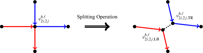

  

  The splitting operation for vertex $v_{2i,2j}^{h,\ell }$ when $(h,\ell )\notin S_{i,j}$. The idea behind this splitting is that no matter which way we orient the undirected dotted edge we cannot go both from left to right and from top to bottom. However, if we just want to go from left to right (top to bottom) then it is possible by orienting the dotted edge to the right (left), respectively

• Splitting Operation We first define the sets $S_{i,j}\subseteq [n]\times [n]$ for each $i,j \in [k]$:

  • For each $i \in [k]$ we let $S_{i,i} = \{(x,x) \mid x\in [n-1]\}$.

  • For each $i,j \in [k]$ with $i \ne j$ we let $S_{i,j} = \{(x,y), (y,x) \mid \{u_x,u_y\} \in E(G')\}$. That is, $S_{i,j}$ represents the ones in the adjacency matrix of $G'$ (with one extra row and one extra column of zeroes added).

  Then for each $i,j\in [k]$ and each $x,y\in [n]$ we perform the following operation on the vertex $v_{2i,2j}^{x,y}$:

  • If $(x,y)\in S_{i,j}$ then we keep the vertex $v_{2i,2j}^{x,y}$ as is.

  • Otherwise we split the vertex $v_{2i,2j}^{x,y}$ into two vertices $v_{2i,2j,\text {LB}}^{x,y}$ and $v_{2i,2j,\text {TR}}^{x,y}$. Note that $v_{2i,2j}^{x,y}$ had 4 incident edges: two incoming (one each from the left and the top) and two outgoing (one each to the right and the bottom). We change the edges as follows (see Fig. 2):

    • Make the left incoming edge and bottom outgoing edge incident on $v_{2i,2j,\text {LB}}^{x,y}$ (denoted by red color in Fig. 2).

    • Make the top incoming edge and right outgoing edge incident on $v_{2i,2j,\text {TR}}^{x,y}$ (denoted by blue color in Fig. 2).

    • Add an undirected edge between $v_{2i,2j,\text {LB}}^{x,y}$ and $v_{2i,2j,\text {TR}}^{x,y}$ (denoted by the dotted edge in Fig. 2).

  By slightly abusing the notation we still refer to the grid as $G_{2i,2j}$, even though some of its vertices were split.

• The set $\mathscr {T}$ of terminal pairs is given by $\bigcup _{i \in [k]} \mathscr {T}_i^{\text {L}} \cup \mathscr {T}_i^{\text {R}} \cup \mathscr {T}_i^{\text {T}} \cup \mathscr {T}_i^{\text {B}} \cup \mathscr {T}_i^{\text {H}} \cup \mathscr {T}_i^{\text {V}}$, where (see also Fig. 3)

  • $\mathscr {T}_j^{\text {L}} = \{(a_{2j-1}^{n}, \widehat{a}_{j}^{1}), (a_{2j-1}^{1}, \widehat{a}_{j}^{n}),(a_{2j}^{1}, \widehat{a}_{j}^{1}), (a_{2j}^{n}, \widehat{a}_{j}^{n})\}$ for each $j\in [k]$,

  • $\mathscr {T}_j^{\text {R}} =\{(\widehat{b}_{j}^{1}, b_{2j-1}^{n}), (\widehat{b}_{j}^{n}, b_{2j-1}^{1}), (\widehat{b}_{j}^{1}, b_{2j}^{1}),(\widehat{b}_{j}^{n}, b_{2j}^{n})\}$ for each $j\in [k]$,

  • $\mathscr {T}_i^{\text {T}} =\{(c_{2i-1}^{n}, \widehat{c}_{i}^{1}), (c_{2i-1}^{1}, \widehat{c}_{i}^{n}),(c_{2i}^{1}, \widehat{c}_{i}^{1}), (c_{2i}^{n}, \widehat{c}_{i}^{n})\}$ for each $i\in [k]$,

  • $\mathscr {T}_i^{\text {B}} =\{(\widehat{d}_{i}^{1}, d_{2i-1}^{n}), (\widehat{d}_{i}^{n}, d_{2i-1}^{1}),(\widehat{d}_{i}^{1}, d_{2i}^{1}),(\widehat{d}_{i}^{n}, d_{2i}^{n})\}$ for each $i\in [k]$,

  • $\mathscr {T}_j^{\text {H}} =\{(a_{2j-1}^{n}, b_{2j-1}^{1}), (a_{2j}^{n}, b_{2j}^{1})\}$ for each $j\in [k]$, and

  • $\mathscr {T}_i^{\text {V}} =\{(c_{2i-1}^{n}, d_{2i-1}^{1}), (c_{2i}^{n}, d_{2i}^{1})\}$ for each $i\in [k]$

Fig. 3

Illustration of the terminal pairs in two consecutive rows. Each pair is represented by a magenta arrow between the appropriate vertices. The black labels represent the sets the pair belongs to, i.e., L stands for $\mathscr {T}_j^{\text {L}}$, R stands for $\mathscr {T}_j^{\text {R}}$, and H stands for $\mathscr {T}_j^{\text {H}}$

Note that the total number of terminal pairs is $(4\cdot 4+2\cdot 2)k= 20k$.

Remark 1

Note that the constructed graph G is planar: Fig. 1 gives a planar embedding of the graph before the splitting operation, and the splitting operation (see Fig. 2) clearly preserves planarity.

Remark 2

Note that the index n does not appear in either first or second coordinate of any pair in the sets $S_{i,j}$ (for any $i,j \in [k]$) as there is no vertex $u_n$ in $G'$. This technical condition is not necessary for our reduction, but we added it to help simplify³ some of the definitions and proofs which appear later in the paper. For example, one can now observe easily that all vertices in $\texttt {Right}(G_{2i,2j})$ and $\texttt {Bottom}(G_{2i,2j})$ are split (for every $i,j\in [k]$).

Before giving an intuition about and proving the properties of the reduction, we first introduce some notation concerning orientations of the green path edges (i.e. potential solutions) of the instance.

Definition 1

For any $i\in [n]$, a path on n vertices $a_1 - a_2 -\cdots - a_n$ is said to be oriented towards (away from) i if every edge $a_{j-1} - a_{j}$ is oriented towards (away from) $a_{j}$ for every $j\le i$ and every edge $a_{j} - a_{j+1}$ is oriented towards (away from) $a_{j}$ for every $j\ge i$, respectively.

We now give some intuition on how the individual terminal pairs enforce the desired structure on the solution (see Figs. 3 and 4). To satisfy pairs in $\mathscr {T}_j^{\text {L}}$ the path $\widehat{A}_j$ must be oriented away from some index, path $A_{2j-1}$ towards the same index and path $A_{2j}$ towards the opposite index (see Lemma 4). Similarly, to satisfy pairs in $\mathscr {T}_j^{\text {R}}$ the path $\widehat{B}_j$ must be oriented towards some index, the path $B_{2j-1}$ must be oriented away from the same index and the path must be oriented $B_{2j}$ away from the opposite index. Then, the pairs in $\mathscr {T}_j^{\text {H}}$ enforce one inequality on the indexes selected on left and right side each, and to satisfy them, there must be a horizontal path from left to right in each row (see Lemma 5). Pairs in $\mathscr {T}_i^{\text {T}}$, $\mathscr {T}_i^{\text {B}}$, and $\mathscr {T}_i^{\text {V}}$ enforce similar properties on paths $\widehat{C}_i$, $C_{2i-1}$, $C_{2i}$, $\widehat{D}_i$, $D_{2i-1}$, $D_{2i}$ and the existence of a vertical path in each column. The splitting in grids on the diagonal enforces that the indexes selected in rows are the same as those selected in the corresponding columns and thus actually correspond to selecting a vertex of $G'$ (see Lemma 6). The splitting in grids off the diagonal ensures that the selected vertices are adjacent (see Lemma 7).

Fig. 4

Illustration of the oriented paths in an intended solution in two consecutive rows of the construction. The arcs used by the paths are drawn in magenta, vertical paths are not drawn. The path $\widehat{A}_j$ is oriented away from $n+1-x_j$ in Lemma 1 and away from $n+1-\lambda _j$ in Lemmas 4 and 6. The path $A_{2j-1}$ is oriented towards $n+1-x_j$ in Lemma 1, towards $n+1-\lambda _j$ in Lemmas 4 and 6, and towards $\alpha _{2j-1}$ in Lemma 5. The path $A_{2j}$ is oriented towards $x_j$ in Lemma 1, towards $\lambda _j$ in Lemmas 4 and 6, and towards $\alpha _{2j}$ in Lemma 5. The path $B_{2j-1}$ is oriented away from $n+1-x_j$ in Lemma 1, away from $n+1-\mu _j$ in Lemmas 4 and 6, and away from $\beta _{2j-1}$ in Lemma 5. The path $B_{2j}$ is oriented away from $x_j$ in Lemma 1, away from $\mu _j$ in Lemmas 4 and 6, and away from $\beta _{2j}$ in Lemma 5. The path $\widehat{B}_j$ is oriented towards $n+1-x_j$ in Lemma 1 and towards $n+1-\mu _j$ in Lemmas 4 and 6

2.2 Completeness of the Reduction

In this subsection we prove the following lemma.

Lemma 1

On an instance $(G',k)$ of k-Clique such that $G'$ contains a clique of size k, the reduction produces an instance $(G,\mathscr {T})$ of Planar Steiner Orientation which has a solution satisfying all terminal pairs.

Suppose that $G'$ has a clique X of size k. Let the clique be formed by the vertices $u_{x_1},u_{x_2}, \ldots ,u_{x_k}$. We know that $x_i \in [n]$ for each $i \in [k]$. We now show that the constructed instance $(G,\mathscr {T})$ of Planar Steiner Orientation has a solution that satisfies all the terminal pairs. Orient the undirected green path edges as follows (see Fig. 4 for an illustration). For each $i,j\in [k]$

• orient $\widehat{A}_j$ and $B_{2j-1}$ away from $n+1-x_j$,

• orient $A_{2j-1}$ and $\widehat{B}_j$ towards $n+1-x_j$,

• orient $A_{2j}$ towards $x_j$,

• orient $B_{2j}$ away from $x_j$,

• orient $\widehat{C}_i$ and $D_{2i-1}$ away from $n+1-x_i$,

• orient $C_{2i-1}$ and $\widehat{D}_i$ towards $n+1-x_i$.

• orient $C_{2i}$ towards $x_i$,

• orient $D_{2i}$ away from $x_i$,

Note that so far we have only oriented the undirected green path edges, and that the dotted undirected edges arising from the splitting operation (Fig. 2) are not yet oriented at this step. It is easy to see that the above orientations ensure that all terminal pairs of $\bigcup _{i \in [k]} \mathscr {T}_i^{\text {L}} \cup \mathscr {T}_i^{\text {R}} \cup \mathscr {T}_i^{\text {T}} \cup \mathscr {T}_i^{\text {B}}$ are satisfied (see Fig. 4). We now show that terminal pairs of $\bigcup _{i \in [k]} \mathscr {T}_i^{\text {H}} \cup \mathscr {T}_i^{\text {V}}$ are also satisfied. First we need some definitions:

Definition 2

(horizontal canonical paths) For $j\in [2k]$ and $\ell \in [n]$, we denote by $Q_{j}^{\ell }$ the unique (horizontal) directed $a_{j}^{\ell } \rightarrow b_{j}^{\ell }$ path whose second vertex is $v_{1,j}^{1,\ell }$ and second-last vertex is $v_{2k,j}^{n,\ell }$ if j is odd and $v_{2k,j,\text {TR}}^{n,\ell }$ if j is even. This path starts with the blue connector edge from $a_{j}^{\ell }$ to $v_{1,j}^{1,\ell }$ and ends with the blue connector edge from $v_{2k,j}^{n,\ell }$ or $v_{2k,j,\text {TR}}^{n,\ell }$ to $b_{j}^{\ell }$. The intermediate edges are obtained by selecting the paths of black edges given by the $\ell$th rows of each gadget $G_{i,j}$ for $i\in [2k]$, and connecting these small paths by horizontal orange edges.

However, we need to address what to do when we encounter a split vertex on this path. Consider the vertex $v_{i,j}^{h,\ell }$ for some $i\in [2k]$ and $h\in [n]$. If $v_{i,j}^{h,\ell }$ is not split, then we do not have to do anything. Otherwise, if $v_{i,j}^{h,\ell }$ is split, then we add the edge $v_{i,j,\text {LB}}^{h,\ell }\rightarrow v_{i,j,\text {TR}}^{h,\ell }$ to $Q_{j}^{\ell }$.

Note that the orientation of G which orients all dotted edges rightwards, i.e., $\text {LB}\rightarrow \text {TR}$, contains each of the horizontal canonical paths defined above.

Definition 3

(vertical canonical paths) For $i\in [2k]$ and $h \in [n]$, we denote by $P_{i}^{h}$ the unique (vertical) $c_i^{h} \rightarrow d_i^{h}$ path whose second vertex is $v_{i,1}^{h,1}$ and second-last vertex is $v_{i,2k}^{h,n}$ if i is odd and $v_{i,2k,\text {LB}}^{h,n}$ if i is even. This path starts with the blue connector edge $(c_{i}^{\ell }, v_{i,1}^{h,1})$ and ends with the blue connector edge from $v_{i,2k}^{h,n}$ or $v_{i,2k,\text {LB}}^{h,n}$ to $d_{i}^{\ell }$. The intermediate edges are obtained by selecting the paths of black edges given by the $\ell$th columns of each gadget $G_{i,j}$ for $j\in [2k]$, and connecting these small paths by vertical orange edges.

However, we need to address what to do when we encounter a split vertex on this path. Consider the vertex $v_{i,j}^{h,\ell }$ for some $j\in [2k]$ and $\ell \in [n]$. If $v_{i,j}^{h,\ell }$ is not split, then we do not have to do anything. Otherwise, if $v_{i,j}^{h,\ell }$ is split, then we add the edge $v_{i,j,\text {LB}}^{h,\ell }\leftarrow v_{i,j,\text {TR}}^{h,\ell }$ to $P_{i}^{h}$.

Note that the orientation of G which orients all dotted edges leftwards, i.e., $\text {LB}\leftarrow \text {TR}$, contains each of the vertical canonical paths defined above. Observe that both the horizontal canonical paths and vertical canonical paths assign orientations to the dotted edges arising from splitting vertices. Hence, one needs to be careful because the splitting operation (see Fig. 2) is designed to ensure that the existence of a horizontal canonical path implies that some vertical canonical path cannot exist (recall that we are allowed to orient each undirected edge in exactly one direction).

Definition 4

(realizable set of paths) A set of directed paths $\mathscr {P}$ in a mixed graph G is realizable if there is an orientation $G^*$ of G such that each path $P\in \mathscr {P}$ appears in $G^*$.

Lemma 2

The set of vertical canonical paths $\{P_{2i-1}^{n+1-x_i}, P_{2i}^{x_i}\mid i\in [k]\}$ together with the set of horizontal canonical paths $\{Q_{2j-1}^{n+1-x_j}, Q_{2j}^{x_j}\mid j\in [k]\}$ are realizable in G.

Proof

Orient each undirected dotted edge which appears on some horizontal path from $\{Q_{2j-1}^{n+1-x_j}, Q_{2j}^{x_j}\mid j\in [k]\}$ in $\text {LB}\rightarrow \text {TR}$ direction and each undirected dotted edge which appears on some vertical path from $\{P_{2i-1}^{n+1-x_i}, P_{2i}^{x_i}\mid i\in [k]\}$ in $\text {TR}\rightarrow \text {LB}$ direction. Since, if $i=j$, then we have $(x_i,x_i) \in S_{i,i}$ by definition and if $i\ne j$, then $u_{x_i}$ and $u_{x_j}$ are adjacent in $G'$ as X is a clique in $G'$, implying that we also have $(x_i,x_j) \in S_{i,j}$ by definition, no black vertex $v_{2i,2j}^{x_i,x_j}$ was split. Thus there is no undirected dotted edge which would appear on both a horizontal and a vertical path from the set. To prove the lemma it remains to arbitrarily orient the edges which do not have a prescribed orientation yet. $\square$

Observe that for each $j\in [k]$, the horizontal path $Q_{2j-1}^{n+1-x_j}$ together with the oriented paths $a_{2j-1}^{n} \rightarrow a_{2j-1}^{n+1-x_j}$ in $A_{2j-1}$ and $b_{2j-1}^{n+1-x_j} \rightarrow b_{2j-1}^{1}$ in $B_{2j-1}$ satisfies the terminal pair $(a_{2j-1}^{n}, b_{2j-1}^{1})$ of $\mathscr {T}_j^{\text {H}}$ for each $j\in [k]$ (see Fig. 4). The same holds for the horizontal path $Q_{2j}^{x_j}$, paths in $A_{2j}$ and $B_{2j}$ and the terminal pair $(a_{2j}^{n}, b_{2j}^{1})$ of $\mathscr {T}_j^{\text {H}}$ for each $j\in [k]$.

Similarly, for each $i\in [k]$, the path $P_{2i-1}^{n+1-x_i}$ together with the oriented paths $c_{2i-1}^{n} \rightarrow c_{2i-1}^{n+1-x_i}$ in $C_{2i-1}$ and $d_{2i-1}^{n+1-x_i} \rightarrow d_{2i-1}^{1}$ in $D_{2i-1}$ satisfies the terminal pair $(c_{2i-1}^{n}, d_{2i-1}^{1})$ of $\mathscr {T}_i^{\text {V}}$. Finally, the path $P_{2i}^{x_i}$ together with paths in $C_{2i}$ and $D_{2i}$ satisfies pair $(c_{2i}^{n}, d_{2i}^{1})$ of $\mathscr {T}_i^{\text {V}}$ for each $i\in [k]$.

Lemma 2 guarantees that these families of canonical vertical and horizontal paths can be realized by some orientation of G (note that the canonical paths only orient black edges, and not green path edges whose orientation was already fixed at the start of this subsection). This implies that $(G,\mathscr {T})$ has a solution which satisfies all terminal pairs, concluding the proof Lemma 1.

2.3 Soundness of the Reduction

In this subsection we prove the following lemma.

Lemma 3

Let $(G',k)$ be an input instance of k-Clique, $(G,\mathscr {T})$ be instance of Planar Steiner Orientation produced by the reduction, and $0 < \vartheta \le \frac{1}{20}$. If there is an orientation $G^*$ of G which satisfies at least $(\frac{19}{20} +\vartheta )$-fraction of the terminal pairs, then there is a clique of size at least $20 \vartheta \cdot k$ in $G'$. In particular, if $G^*$ satisfies all terminal pairs, then $G'$ has a clique of size k.

Let $G^*$ be the orientation which satisfies at least $(\frac{19}{20} +\vartheta )$-fraction of terminal pairs from $\mathscr {T}$. Note that the set of vertices $A\cup \widehat{B}\cup C\cup \widehat{D}$ has no incoming edges. Similarly, the set of vertices $\widehat{A}\cup B\cup \widehat{C}\cup D$ has no outgoing edges.

The next lemma restricts the orientations of the undirected paths of green path edges.

Lemma 4

In the orientation $G^*$, for each $i,j\in [k]$ we have that

• if $G^*$ satisfies all pairs of $\mathscr {T}_j^{\text {L}}$, then there exists an integer $\lambda _j \in [n]$ such that the path $\widehat{A}_{j}$ is oriented away from $n+1-\lambda _j$, the path $A_{2j-1}$ is oriented towards $n+1-\lambda _j$ and the path $A_{2j}$ is oriented towards $\lambda _j$.

• if $G^*$ satisfies all pairs of $\mathscr {T}_j^{\text {R}}$, then there exists an integer $\mu _j \in [n]$ such that the path $\widehat{B}_{j}$ is oriented away from $n+1-\mu _j$, the path $B_{2j-1}$ is oriented away from $n+1-\mu _j$ and the path $B_{2j}$ is oriented towards $\mu _j$.

• if $G^*$ satisfies all pairs of $\mathscr {T}_i^{\text {T}}$, then there exists an integer $\delta _i \in [n]$ such that the path $\widehat{C}_{i}$ is oriented away from $n+1-\delta _i$, the path $C_{2i-1}$ is oriented towards $n+1-\delta _i$ and the path $C_{2i}$ is oriented towards $\delta _i$.

• if $G^*$ satisfies all pairs of $\mathscr {T}_i^{\text {B}}$, then there exists an integer $\varepsilon _i \in [n]$ such that the path $\widehat{D}_{i}$ is oriented away from $n+1-\varepsilon _i$, the path $D_{2i-1}$ is oriented away from $n+1-\varepsilon _i$ and the path $D_{2i}$ is oriented towards $\varepsilon _i$.

Proof

Fix $j\in [k]$. We just prove the lemma for the pairs of $\mathscr {T}_j^{\text {L}}$ and the paths $\widehat{A}_{j}$, $A_{2j-1}$, and $A_{2j}$ since the proof for other cases is similar. See again Fig. 4 for an illustration. Since the only edges incoming to $\widehat{A}$ are blue connector edges from A (and A has no incoming edges), it follows that the terminal pairs $(a_{2j-1}^{n}, \widehat{a}_{j}^{1})$ and $(a_{2j-1}^{1}, \widehat{a}_{j}^{n})$ of $\mathscr {T}_j^{\text {L}}$ are satisfied by edges from the graph $G^{*}[\widehat{A}_j \cup A_{2j-1}]$. The path satisfying the terminal pair $(a_{2j-1}^{n}, \widehat{a}_{j}^{1})$ has to travel upwards along $A_{2j-1}$, use a blue connector edge and then finally travel upwards along $\widehat{A}_j$. Similarly, the path satisfying the terminal pair $(a_{2j-1}^{1}, \widehat{a}_{j}^{n})$ has to travel downwards along $A_{2j-1}$, use a blue connector edge and then finally travel downwards along $\widehat{A}_j$. Since we can only orient each green path edge in exactly one direction, it follows that both these paths must use the same blue connector edge, i.e., there exists an integer $\lambda '_i \in [n]$ such that the paths $\widehat{A}_j, A_{2j-1}$ are oriented away from, and towards $\lambda '_i$, respectively. A similar argument shows that both the paths satisfying the terminal pairs $(a_{2j}^{1}, \widehat{a}_{j}^{1})$ and $(a_{2j}^{n}, \widehat{a}_{j}^{n})$ have to use the blue connector edge $a_{2j}^{n+1-\lambda '_i} \rightarrow \widehat{a}_{j}^{\lambda '_i}$. Hence, the path $A_{2j}$ is oriented towards $n+1-\lambda '_i$. Setting $\lambda _i=n+1-\lambda '_i$, we obtain the desired result. $\square$

Lemma 5

Let $G^*$ be an orientation of G. For each $j\in [2k]$ if $A_j$ is oriented towards $\alpha _j \in [n]$, path $B_j$ is oriented away from $\beta _j \in [n]$, and the pair $(a_{j}^{n}, b_{j}^{1})$ is satisfied in $G^*$, then $\alpha _j \le \beta _j$. If moreover $\alpha _j = \beta _j$, then $G^*$ contains the horizontal canonical path $Q_{j}^{\alpha _j}$.

For each $i\in [2k]$ if $C_i$ is oriented towards $\gamma _i \in [n]$, path $D_i$ is oriented away from $\zeta _i \in [n]$, and the pair $(c_{i}^{n}, b_{i}^{1})$ is satisfied in $G^*$, then $\gamma _i \le \zeta _i$. If moreover $\gamma _i = \zeta _i$, then $G^*$ contains the vertical canonical path $P_{i}^{\gamma _i}$.

Proof

We only prove the first two claims, the proof for the other two is completely analogous. See again Fig. 4 for an illustration. Fix any $j\in [2k]$ and consider the terminal pair $(a_{j}^{n}, b_{j}^{1})$. Since $G^*$ satisfies the pair $(a_{j}^{n}, b_{j}^{1})$, it contains a path P from $a_{j}^{n}$ to $b_{j}^{1}$. Since $\widehat{A}$ has no outgoing edges, P does not contain any vertices of $\widehat{A}$. Similarly, P does not contain any vertices of $\widehat{B}$. Hence, the path P consist of the following five parts: the vertical upwards path $a_{j}^{n}\rightarrow a_{j}^{n-1}\rightarrow \cdots \rightarrow a_{j}^{\tau }$ followed by the blue connector edge $a_{j}^{\tau }\rightarrow v_{1,j}^{1,\tau }$, then a path in the graph $G^{*}\Big [\bigcup _{i=1}^{2k}\bigcup _{j'=1}^{2k} V(G_{i,j'})\Big ]$ followed by a blue connector edge $v_{2k,j}^{n,\upsilon }\rightarrow b_{j}^{\upsilon }$ and a vertical upwards path $b_{j}^{\upsilon } \rightarrow b_{j}^{\upsilon -1} \cdots \rightarrow b_{j}^{1}$. If j is even, then the second blue connector edge is actually $v_{2k,j,\text {TR}}^{n,\upsilon }\rightarrow b_{j}^{\upsilon }$.

Since $A_j$ is oriented towards $\alpha _j$, for the first part of P to exist we have $\alpha _j \le \tau$. Similarly, since $B_j$ is oriented away from $\beta _j$, we have $\upsilon \le \beta _j$. Furthermore, all edges in $G^{*}\Big [\bigcup _{i=1}^{2k}\bigcup _{j'=1}^{2k} V(G_{i,j'})\Big ]$, except for those formed by splitting vertices, are oriented either downward or to the right. Moreover, the splitting does not really change the row/column level. Therefore, the central part of P only goes down or right and $\tau \le \upsilon$. Together we obtain $\alpha _j \le \tau \le \upsilon \le \beta _j$, and the first claim follows.

Moreover, if $\alpha _j = \beta _j$, then $\tau = \upsilon =\alpha _j$ and the central part of P only goes right and from $\text {LB}$ to $\text {TR}$ within the split vertices. It follows that it is the horizontal canonical path $Q_{j}^{\alpha _j}$. $\square$

Lemma 6

For each $i\in [k]$ and $j \in [k]$ and integers $\lambda _j$, $\mu _j$, $\delta _i$, $\varepsilon _i$ as given by Lemma 4 we have the following.

• If $G^*$ satisfies all pairs in $\mathscr {T}_j^{\text {L}} \cup \mathscr {T}_j^{\text {R}} \cup \mathscr {T}_j^{\text {H}}$, then $\lambda _j = \mu _j$. Moreover, $G^*$ contains the horizontal canonical path $Q_{2j}^{\lambda _j}$.

• If $G^*$ satisfies all pairs in $\mathscr {T}_i^{\text {T}} \cup \mathscr {T}_i^{\text {B}} \cup \mathscr {T}_i^{\text {V}}$, then $\delta _i = \varepsilon _i$. Moreover, $G^*$ contains the vertical canonical path $P_{2i}^{\delta _i}$.

• If $i=j$ and both previous conditions hold, then moreover $\lambda _i=\delta _i$.

Proof

Fix $j\in [k]$. See again Fig. 4 for an illustration. We first prove that $\lambda _j = \mu _j$, if $G^*$ satisfies the pairs in $\mathscr {T}_j^{\text {L}} \cup \mathscr {T}_j^{\text {R}} \cup \mathscr {T}_j^{\text {H}}$. In this case, by Lemma 4, $A_{2j-1}$ is oriented towards $n+1-\lambda _j$ and $B_{2j-1}$ is oriented away from $n+1-\mu _j$ and from Lemma 5 it follows that $n+1-\lambda _j \le n+1-\mu _j$. That is, $\lambda _j \ge \mu _j$. Since $A_{2j}$ is oriented towards $\lambda _j$ and $B_{2j}$ is oriented away from $\mu _j$, from Lemma 5 it follows that $\lambda _j \le \mu _j$. Thus $\lambda _j = \mu _j$ and applying Lemma 5 again to paths $A_{2j}$ and $B_{2j}$ we get that $G^*$ contains the horizontal canonical path $Q_{2j}^{\lambda _j}$.

The proof for the second part is completely analogous to the proof of the first part. Thus we move to the third part. From the previous two parts we know that $G^*$ contains both the the horizontal canonical path $Q_{2i}^{\lambda _i}$ and the vertical canonical path $P_{2i}^{\delta _i}$. It follows that the vertex $v_{2i,2i}^{\delta _i,\lambda _i}$ was not split, that is $(\delta _i,\lambda _i) \in S_{i,i}$. This implies $\delta _i=\lambda _i$ by the definition of $S_{i,i}$, concluding the proof. $\square$

Definition 5

An index $i \in [k]$ is called good (for $G^*$) if all terminal pairs from $\mathscr {T}_i^{\text {L}} \cup \mathscr {T}_i^{\text {R}} \cup \mathscr {T}_i^{\text {T}} \cup \mathscr {T}_i^{\text {B}} \cup \mathscr {T}_i^{\text {H}} \cup \mathscr {T}_i^{\text {V}}$ are satisfied in $G^*$.

Lemma 7

If both $i,j \in [k]$, $i \ne j$ are good in $G^*$, then $\{u_{\delta _i},u_{\delta _j}\} \in E(G')$. In particular $\delta _i \ne \delta _j$.

Proof

By Lemma 6, if i, j are good, then $G^*$ contains the horizontal canonical path $Q_{2j}^{\delta _j}$ and the vertical canonical path $P_{2i}^{\delta _i}$. It follows that the vertex $v_{2i,2j}^{\delta _i,\delta _j}$ was not split, that is $(\delta _i,\delta _j) \in S_{i,j}$. This implies $\{u_{\delta _i},u_{\delta _j}\} \in E(G')$ by the definition of $S_{i,j}$. The second part follows as we do not allow loops. $\square$

Lemma 8

Let $Y \subseteq [k]$ be the set of good indices. For each $0\le \vartheta \le \frac{1}{20}$, if $G^*$ satisfies at least $(\frac{19}{20} +\vartheta )$-fraction of the terminal pairs, then $|Y| \ge 20\vartheta \cdot k$.

Proof

If i is good then all 20 pairs from $\mathscr {T}_i^{\text {L}} \cup \mathscr {T}_i^{\text {R}} \cup \mathscr {T}_i^{\text {T}} \cup \mathscr {T}_i^{\text {B}} \cup \mathscr {T}_i^{\text {H}} \cup \mathscr {T}_i^{\text {V}}$ are satisfied in $G^*$. Otherwise, at most 19 pairs from this set are satisfied. Hence, the total number of satisfied pairs is at most $20|Y|+19(k-|Y|)= 19k+|Y|$. However, we know that $G^*$ satisfies at least $(\frac{19}{20} +\vartheta )|\mathscr {T}|=(\frac{19}{20} +\vartheta )20k=19k+20\vartheta \cdot k$ pairs. Hence, we have $|Y| \ge 20\vartheta \cdot k$. $\square$

Proof of Lemma 3

If $G^*$ satisfies at least $(\frac{19}{20} +\vartheta )$-fraction of the terminal pairs, then by Lemma 8 there is a set Y of good indices of size at least $20\vartheta \cdot k$. By Lemma 7 the set $X=\{u_{\delta _i} \mid i \in Y\}$ forms a clique in $G'$ of size at least $20\vartheta \cdot k$.

2.4 Proving the Lower Bounds

In this subsection we finish the proof of both our theorems.

Proof of Theorem 1

It is easy to see that the graph G has $O(n^{2}k^{2})$ vertices and can be constructed in $\text {poly}(n+k)$ time. Recall that (Remark 1) the graph G constructed in the Steiner Orientation instance is planar. Combining this with the two directions from Lemmas 1 and 3, we get a parameterized reduction from k-Clique to Planar Steiner Orientation. Hence, the W[1]-hardness of Planar Steiner Orientation follows from the W[1]-hardness of k-Clique. Chen et al. [4] showed that, for any function f, the existence of an $f(k)\cdot n^{o(k)}$ algorithm for k-Clique violates ETH. Our reduction transforms an instance of k-Clique into an equivalent instance of Planar Steiner Orientation with O(k) demand pairs. We obtain that under ETH there is no $f(k)\cdot n^{o(k)}$ time algorithm for Planar Steiner Orientation. This concludes the proof.

For the inapproximability proof we need some more definitions. We will use the recent result on parameterized inapproximability of k-Clique from [3]. To state the result precisely, let us first state the underlying assumption, the Gap Exponential Time Hypothesis (Gap-ETH).

Hypothesis 1

((Randomized) Gap-ETH [11, 16]) There exists a constant $\delta > 0$ such that, given a 3CNF formula $\varPhi$ on n variables, no (possibly randomized) $2^{o(n)}$-time algorithm can distinguish between the following two cases correctly with probability at least 2/3:

• $\varPhi$ is satisfiable.

• Every assignment to the variables violates at least a $\delta$-fraction of the clauses of $\varPhi$.

Here we do not attempt to reason why Gap-ETH is a plausible assumption; for more detailed discussions on the topic, please refer to [11] or [3]. For now, let us move on to state the inapproximability result from [3] that we need. Chalermsook et al. [3] showed that the only way to distinguish graphs with large cliques from those with small cliques is essentially to enumerate all vertex subsets of certain size, as stated more formally below.

Theorem 3

([3, Theorem 18]) Assuming Gap-ETH, there exist constants $\delta , r_0 > 0$ such that, for any function g and for any positive integers $q \ge r \ge r_0$, there is no algorithm that, given a graph $G'$, can distinguish between the following cases in $g(q,r)\cdot n^{\delta r}$ time, where $n=|V(G')|$:

• $\textsc {Clique}(G') \ge q$ and

• $\textsc {Clique}(G') < r$,

where $\textsc {Clique}(G')$ denotes the maximum size of a clique in $G'$.

While the construction presented in [3] is randomized, the authors claim that it can be derandomized so that the assumption can be limited to the (deterministic) Gap-ETH.

Proof of Theorem 2

Let $\delta$ and $r_0$ be the constants from Theorem 3, $\vartheta$ be a constant such that $0<\vartheta \le \frac{1}{20}$ and let $\zeta =\frac{\vartheta \delta }{4}$. Let $r=\max \{3,r_0\}$ and $q=\lceil \frac{r}{20\vartheta }\rceil$. Note that since $r > 2$, we have $q >2$ and, thus $q \le 2\frac{r}{20\vartheta }$.

Assume for contradiction that there is a function f and an algorithm $\mathbb {A}$ that can distinguish between the two cases:

• there is an orientation of G that satisfies all pairs of $\mathscr {T}$ and

• any orientation of G satisfies less than $\frac{19}{20} + \vartheta$ fraction of pairs in $\mathscr {T}$

in $f(|\mathscr {T}|)(|V(G)|^{\zeta |\mathscr {T}|})$ time.

We design an algorithm $\mathbb {B}$ that will contradict Theorem 3 for q and r as follows. Given a graph $G'$ we apply our reduction from Sect. 2.1 to the instance $(G',q)$ of Clique. Then we apply algorithm $\mathbb {A}$ to the resulting instance $(G,\mathscr {T})$ of Steiner Orientation. If $G'$ contains a clique of size q, then, by Lemma 1, there is an orientation of G satisfying all pairs from $\mathscr {T}$ and the algorithm $\mathbb {A}$ recognizes that. If each clique in $G'$ is of size less than $r\le 20\vartheta q$, then each orientation of G satisfies less than a $\frac{19}{20} + \vartheta$ fraction of pairs in $\mathscr {T}$. Indeed, by Lemma 3, if any orientation satisfied a $\frac{19}{20} + \vartheta$ fraction of pairs in $\mathscr {T}$, then there would be a clique of size $20\vartheta q \ge r$ in $G'$. Again, the algorithm $\mathbb {A}$ recognizes that.

Now since $|V(G)|=O(q^2|V(G')|^2)$, the reduction can be performed in linear time in the size of the output, and $\mathbb {A}$ runs in time $f(|\mathscr {T})|(|V(G)|^{\zeta |\mathscr {T}|})$, we obtain that $\mathbb {B}$ runs in time

$$\begin{aligned}&f(|\mathscr {T}|)(|V(G)|^{\zeta |\mathscr {T}|})= f(20q)((O(q^2|V(G')|^2))^{\zeta \cdot 20q})\\&\quad =f(20q)((O(q^2))^{\zeta \cdot 20q})(|V(G')|^2)^{\zeta \cdot 20q})= g(q)(|V(G')|^{2\cdot \zeta \cdot 20q})\le g(q)(|V(G')|^{\delta \cdot r}), \end{aligned}$$

for suitable g. The last inequality holds since $2\zeta \cdot 20q = 2\zeta \cdot 20 \cdot \lceil \frac{r}{20\vartheta }\rceil \le 2\zeta \cdot 20 \cdot 2\frac{r}{20\vartheta }= \frac{4\zeta }{\vartheta }r=\frac{4\vartheta \delta }{4\vartheta }r=\delta r$ by the definition of $\zeta$.

Thus the existence of $\mathbb {A}$ would indeed contradict Theorem 3. $\square$

3 Open Problems

This work completely closes the gap between upper and lower bounds for the Steiner Orientation problem parameterized by the number of terminal pairs k, even on planar graphs. However, there are still some interesting open questions to pursue. We list some of them below:

• Does Steiner Orientation belong to the class W[1]?

• Can we show W[2]-hardness for Steiner Orientation parameterized by k?

• Can we obtain O(1)-FPT approximation for Planar Steiner Orientation parameterized by k?

References

Arkin, E.M., Hassin, R.: A note on orientations of mixed graphs. Discrete Appl. Math. 116(3), 271–278 (2002)
Beck, M., Blum, J., Kryven, M., Löffler, A., Zink, J.: Planar Steiner Orientation is NP-Complete. CoRR. ar**v:1804.07496 (2018)
Chalermsook, P., Cygan, M., Kortsarz, G., Laekhanukit, B., Manurangsi, P., Nanongkai, D., Trevisan, L.: From gap-ETH to FPT-inapproximability: clique, dominating set, and more. In: FOCS 2017, pp. 743–754 (2017)
Chen, J., Huang, X., Kanj, I.A., **a, G.: Strong computational lower bounds via parameterized complexity. J. Comput. Syst. Sci. 72(8), 1346–1367 (2006)
Chitnis, R., Esfandiari, H., Hajiaghayi, M.T., Khandekar, R., Kortsarz, G., Seddighin, S.: A tight algorithm for strongly connected Steiner subgraph on two terminals with demands. Algorithmica 77(4), 1216–1239 (2017)
Chitnis, R., Feldmann, A.E.: A tight lower bound for Steiner orientation. In: CSR 2018, pp. 65–77 (2018)
Chitnis, R., Feldmann, A.E., Manurangsi, P.: Parameterized approximation algorithms for bidirected Steiner network problems. In: 26th Annual European Symposium on Algorithms, ESA 2018, August 20–22, 2018, Helsinki, Finland, pp. 20:1–20:16 (2018)
Chitnis, R.H., Hajiaghayi, M., Marx, D.: Tight bounds for planar strongly connected Steiner subgraph with fixed number of terminals (and extensions). In: Proceedings of the Twenty-Fifth Annual ACM-SIAM Symposium on Discrete Algorithms, SODA 2014, Portland, Oregon, USA, January 5–7, 2014, pp. 1782–1801 (2014)
Cygan, M., Fomin, F.V., Kowalik, L., Lokshtanov, D., Marx, D., Pilipczuk, M., Pilipczuk, M., Saurabh, S.: Parameterized Algorithms. Springer, Berlin (2015)
Cygan, M., Kortsarz, G., Nutov, Z.: Steiner forest orientation problems. SIAM J. Discrete Math. 27(3), 1503–1513 (2013)
Dinur, I.: Mildly exponential reduction from gap 3SAT to polynomial-gap label-cover. Electron. Colloq. Comput. Complex. (ECCC) 23, 128 (2016)
Gamzu, I., Segev, D., Sharan, R.: Improved orientations of physical networks. In: International Workshop on Algorithms in Bioinformatics (WABI), pp. 215–225 (2010)
Hassin, R., Megiddo, N.: On orientations and shortest paths. Linear Algebra Appl. 114, 589–602 (1989). (special issue dedicated to Alan J. Hoffman)
Impagliazzo, R., Paturi, R.: On the complexity of k-SAT. J. Comput. Syst. Sci. 62(2), 367–375 (2001)
Impagliazzo, R., Paturi, R., Zane, F.: Which problems have strongly exponential complexity? J. Comput. Syst. Sci. 63(4), 512–530 (2001)
Manurangsi, P., Raghavendra, P.: A birthday repetition theorem and complexity of approximating dense CSPs. In: ICALP, pp. 78:1–78:15 (2017)
Marx, D.: On the optimality of planar and geometric approximation schemes. In: 48th Annual IEEE Symposium on Foundations of Computer Science (FOCS 2007), October 20–23, 2007, Providence, RI, USA, Proceedings, pp. 338–348 (2007)
Marx, D.: Can you beat treewidth? Theory Comput. 6(1), 85–112 (2010)
Marx, D.: A tight lower bound for planar multiway cut with fixed number of terminals. In: ICALP (1), pp. 677–688 (2012)
Marx, D., Pilipczuk, M.: Everything you always wanted to know about the parameterized complexity of subgraph isomorphism (but were afraid to ask). In: 31st International Symposium on Theoretical Aspects of Computer Science (STACS 2014), STACS 2014, March 5–8, 2014, Lyon, France, pp. 542–553 (2014)
Marx, D., Pilipczuk, M.: Optimal parameterized algorithms for planar facility location problems using voronoi diagrams. In: Algorithms—ESA 2015—23rd Annual European Symposium, Patras, Greece, September 14–16, 2015, Proceedings, pp. 865–877 (2015)
Medvedovsky, A., Bafna, V., Zwick, U., Sharan, R.: An algorithm for orienting graphs based on cause-effect pairs and its applications to orienting protein networks. In: International Workshop on Algorithms in Bioinformatics (WABI), pp. 222–232 (2008)
Pilipczuk, M., Wahlström, M.: Directed multicut is W[1]-hard, even for four terminal pairs. In: Proceedings of the Twenty-Seventh Annual ACM-SIAM Symposium on Discrete Algorithms, SODA 2016, Arlington, VA, USA, January 10–12, 2016, pp. 1167–1178 (2016)
Pilipczuk, M., Wahlström, M.: Directed multicut is W[1]-hard, even for four terminal pairs. TOCT 10(3), 13:1–13:18 (2018)
Robbins, H.E.: A theorem on graphs, with an application to a problem of traffic control. Am. Math. Mon. 46(5), 281–283 (1939)
Acknowledgements
We would like to thank the reviewers of both CSR’18 and of this version for their detailed and insightful comments which have greatly helped the presentation and readability.
Author information
Authors and Affiliations
Corresponding author
Additional information
Publisher's Note
Springer Nature remains neutral with regard to jurisdictional claims in published maps and institutional affiliations.
A preliminary version of this article [6] showing the W[1]-hardness and the \(f(k)\cdot n^{o(k)}\) running time lower bound under ETH for graphs of genus 1 appeared in CSR’18. This version extends the results to graphs of genus 0 (planar graphs) and also contains an FPT inapproximability result.
Rajesh Chitnis: Supported by ERC Grant CoG 647557 “Small Summaries for Big Data”. Part of this work was done when the author was at the Weizmann Institute of Science (and supported by Israel Science Foundation Grant #897/13), and visiting Charles University in Prague, Czechia.
Andreas Emil Feldmann: Supported by Project CE-ITI (GAČR No. P202/12/G061) of the Czech Science Foundation, and by the Center for Foundations of Modern Computer Science (Charles Univ. Project UNCE/SCI/004).
Ondřej Suchý: Supported by Grant 17-20065S of the Czech Science Foundation.
Rights and permissions
Open Access This article is distributed under the terms of the Creative Commons Attribution 4.0 International License (http://creativecommons.org/licenses/by/4.0/), which permits unrestricted use, distribution, and reproduction in any medium, provided you give appropriate credit to the original author(s) and the source, provide a link to the Creative Commons license, and indicate if changes were made.
About this article
Cite this article
Chitnis, R., Feldmann, A.E. & Suchý, O. A Tight Lower Bound for Planar Steiner Orientation. Algorithmica 81, 3200–3216 (2019). https://doi.org/10.1007/s00453-019-00580-x
Received:
Accepted:
Published:
Issue Date:
DOI: https://doi.org/10.1007/s00453-019-00580-x