The Utility of Socioeconomic and Remoteness Indicators in Understanding the Geographical Variation in the Regional Prevalence of Early Childhood Vulnerability in Australia

Abstract

The family lives of children and their early childhood development outcomes are attributable to the level of socio-economic disadvantage and relative isolation. This study aims to investigate how the disadvantage of the local area (i.e., socio-economic indexes for areas (SEIFA)) and the remoteness (i.e., accessibility/remoteness index of Australia (ARIA)) contribute to improved prevalence estimates of child development vulnerability in statistical areas level 3 (SA3) and 4 (SA4) across Australia. Data from the 2018 Australian Early Development Census (AEDC) has been used. The study included 308,953 children involved in the AEDC 2018 where one-in-ten of them were considered to be developmentally vulnerable, nationally. We developed models in a hierarchical Bayesian framework at the SA3 level using SEIFA and ARIA indices as covariates to account for spatial and unobserved heterogeneity. The performances of developed models are examined based on the consistency at SA3, SA4, and state level. The results reveal that SEIFA makes a significant contribution to explaining the spatial variation in childhood development vulnerability across small domains in Australia. Further, the inclusion of the ARIA score improves the model performance and provides better accuracy, particularly in remote and very remote regions. In these regions, the spatial model fails to distinguish the remoteness characteristics. The chosen non-spatial model accounting for heterogeneity at higher hierarchies performs best. The utilization of socio-economic disadvantage and geographic remoteness of the finer level domains helps to explain the geographic variation in child development vulnerability, particularly in sparsely populated remote regions in Australia.

1 Introduction

1.1 Motivation

The importance of early childhood development in laying the foundations for children’s ongoing physical, emotional, and social development, well into adulthood cannot be underplayed (Sampson et al., 1999). At an individual level, poor early childhood development can increase the prevalence of behavioural problems, affect school enrolment and participation and impair educational attainment (Bronfenbrenner, 1979). At a neighbourhood level, wider inequities in child development may arise due to persistent under- and unemployment, long term mental health issues, poorer health outcomes and higher mortality rates (Sampson et al., 2002; Brooks-Gunn & Duncan, 1977; Leventhal & Brooks-Gunn, 2000), and poor early development and vulnerability is a manifestation of child poverty. It is now recognized that there exists a combined and accumulating effect of poverty on the critical stage of developmental vulnerability and potential (i.e., early childhood) (Brooks-Gunn & Duncan, 1977). Poor early childhood development therefore has implications for health and wellbeing in later life, but also presents a considerable burden for families and the wider society.

While early childhood development is influenced by numerous factors, the role of neighbourhood has been proven to be important. In particular, there is a well-established link between early childhood development outcomes and neighbourhood disadvantage. This neighbourhood disadvantage varies geographically. By and large, researchers have shown that in disadvantaged communities, a lack of resources and opportunities can have adverse contributions to early childhood development outcomes. More pertinently, with strong associations between geographic disadvantage (which manifests as social exclusion or relative isolation) and development outcomes, these poor outcomes can persist from one generation to the next (Aizer & Currie, 2014; Tanton et al., 2012; Vera-Toscano, 2020). In this study we have examined the spatial patterns in childhood development vulnerability in Australian regions, and ascertains how socio-economic disadvantage and the level of geographic isolation elucidates the disparities in the prevalence of childhood developmental vulnerability at a regional level.

Australia is, by world standards, a prosperous nation with a healthy and well educated population who have relatively high economic and social wellbeing. Yet there are a number of subpopulations in the country that are significantly not as well off as the others. Wealth is distributed unevenly. Furthermore, there is a growing disparity in income and wealth with a widening gap between the richest and the poorest in Australian society. Relatedly, people living in Australia’s rural and remote regions experience high rates of poverty. There are also substantial differences in socio-economic, health and outcomes when compared with those living in metropolitan areas, and this has worsened in the last few decades (Adair & Lopez, 2020; Cheers, 1990; Wakerman et al., 2008). The settlement patterns and population distribution, with 80 per cent living along the coastline between Adelaide and Brisbane (on an area roughly 3 per cent of the country’s land mass), speaks volumes about the relative isolation faced by remote communities.

The experience of poverty is closely intertwined with where people live, and the local resources available to them, and as such it is compounded for people in rural and remote areas. When comparing Indigenous and non-Indigenous population, there are significant inequities in many markers of socio-economic advantage, including education, employment, and housing. Inequalities experienced by Aboriginal and Torres Strait Islander people, though well recognised, are persistent and reflected in unacceptably high rates of many preventable conditions and mortality gaps between Indigenous and other Australians (Phillips et al., 2017; Vos et al., 2009; Wilson et al., 2019). However, roughly 70 per cent of Australia’s Aboriginal and Torres Strait Islander people live outside capital cities. In contrast, for non-Indigenous people this figure is 2 per cent (AIHW, 2022a). Inequities in access and service provision mean that disadvantaged communities in Australia often have social and economic characteristics which lead to them being under-resourced and socially excluded from opportunities needed to support good early development outcomes. Our research facilitates a better grasp of the complex underlying mechanisms that lead to disparities between Indigenous and non-Indigenous populations. These disparities point to systemic and historical issues such as dispossession of traditional lands, forced assimilation and separation from family and social networks, and racism and marginalisation (Anderson et al., 2006; Paradies, 2016).

Our study makes two important contributions. Firstly, we provide improved prevalence estimates of children who are considered to be developmentally vulnerable in regions across Australia, through accounting for both socio-economic disadvantage and remoteness. We apply small area estimation methods to provide precise and reliable estimates of regional level childhood vulnerability, offering valuable insights into the spatial diversity of disadvantage and accessibility in Australia. Second, much of the literature that examines the impact of isolation and socio-economic disadvantage uses a combined measure of social exclusion (for example, Exeter et al., 2017; Figari, 2012; Jordan et al., 2004; Noble et al., 2006; Whelan & Maître, 2005).

In our paper, we combine the index for socio-economic disadvantage and the index of remoteness/accessibility to provide a more refined measure of disadvantage, and demonstrate this through early childhood vulnerability in Australia. Through differentiating between two aspects of disadvantage, namely economic and geographical, we facilitate the examination of the relative contributions of these different factors to disadvantage. In addition, we contribute to the wider discussion on the influence of spatial advantage on understanding inequalities, particularly around the spatial influences on the transmission of disadvantage.

1.2 Spatial Disadvantage

Reflecting its origins in urban studies, spatial disadvantage has focused primarily in inner cities, due perhaps to the initial conceptual framework based on how cities are structured into different spatial areas. The premise was that social disadvantage and inequality was reflected in the socio-spatial structure of cities (Timms, 1971; Wilson, 2012). Whereas this holds in deprived ghettos in most developed countries in Europe and America (Massey et al., 2009; Van Ham et al., 2014) and, to a certain extent, in slums of Asia and Africa (Abascal et al., 2022), in Australia, spatial disadvantage is more of an outer-urban problem.

In this context, spatial disadvantage is a manifestation of residential differentiation, where people who live in an area experience concentrations of poverty (including income and housing), disadvantage in resource access (such as employment, education and health), and social problems (for instance, crime, drug addiction, and anti-social behaviours). It is in areas where all three forms of disadvantage coalesce that permanent or sustained spatial disadvantage occurs (Hunter & Gregory, 1996; Manley et al., 2020). Relatedly, there is a complex manner in which socio-economic and spatial inequalities are intertwined.

The context in which spatial disadvantage plays out in different countries reflects a whole range of environmental, economic, and political factors. On the one hand, much of the public debate has focused on the historical concentration of poverty in inner city, metropolitan areas. On the other hand, the trend in Australia is opposite, with a surburbanisation of poverty, and consequently spatial disadvantage is now increasingly an outer-metropolitan problem (Burke & Hulse, 2015; Badcock, 1997).

In this paper we aim to capture spatial disadvantage in regional estimates of early childhood developmental vulnerability. We do this through model-based estimation that includes both measures of socio-economic disadvantage and relative isolation. Through doing this, we aim to understand the spatial variation in the prevalence of regional vulnerability in Australia. Regional differences in spatial disadvantage provide insights into the complex environmental and structural issues through which inter-generational transmission of disadvantage might occur. In particular, it is of interest to determine whether communities with specific spatial characteristics produce vulnerable children who follow similar patterns of poor outcomes in later life.

1.3 Australian Remoteness and Disadvantage

The geographical population distribution of Australia is highly uneven and characterised by both significant levels of urbanisation, and highly sparsely populated remote outback areas. One third of Australia’s population lives outside its major cities (ABS, 2008b). Of this non-metropolitan population, almost twenty percent is dispersed across more than 1,500 rural and remote communities with fewer than 5,000 residents. Collectively these communities have a population the size of Sydney, Australia’s largest city. Furthermore, almost three-quarters of these small communities lie in the rural and remote areas furthest from large population centres (AIHW, 2008).

Remote areas in Australia are characterized by their low population density, large territorial boundaries and relative inaccessibility of population settlements.

There are also diverse demographic differences between metropolitan cities and remote communities, by age, gender and ethnic compositions, as well as by socio-economic and health characteristics. These Australians face unique challenges due to their geographic location. In fact, there is growing evidence (AIHW, 2015; Baade et al., 2011; Burke & Hulse, 2015; Turrell et al., 2006; Wilkinson et al., 2001)

that spatial isolation and lack of connectivity plays a pivotal role in how remote areas are socially vulnerable and spatially disadvantaged. While socio-economic disadvantage and remoteness are unlikely to be the only determinants of area level variation across Australia, they invariably have large contributions, and this research demonstrates the impact of socio-economic gradients and remoteness accessibility on capturing spatial variation in health outcomes.

The experience of disadvantage is closely connected to where people live and the local resources available to them. This implies that poverty in rural and remote Australia has a particular set of characteristics which differentiates it from other jurisdictions. In the main, people in remote areas tend to have lower incomes, experience economic hardship and declining employment opportunities, have reduced access to services such as health, education and transport and live in isolated communities (AIHW, 2008). Furthermore, a significant proportion of Aboriginal and Torres Strait Islander people live outside the capital cities and for those living on low income the experience is exacerbated by specific cultural, language and life experience issues (Paradies et al., 2015; Priest et al., 2011). Indigenous Australians have higher hospitalisation rates, poorer self-reported health, higher burden of disease, higher prevalence of risky health behaviour, and lower life expectancies than non-Indigenous Australians (AIHW, 2022b).

Studies on the spatial features of disadvantage are made more difficult because of the assumption underlying the definition of socio-economic disadvantage (Townsend, 1979) at an areal level. However, disadvantaged people can live in the same neighbourhoods as affluent people (Burke & Hulse, 2015). Aggregating individual measures of socio-economic position such as income, education and employment to capture neighbourhood disadvantage (e.g., % of residents earning under 50% of median income, % of residents without a Bachelor’s degree, or % of residents that own a car) can mask the impact of individual socio-economic disadvantage (Jordan et al., 2004). Recently, in the context of the COVID-19 pandemic, health impacts have been more severe for those with underlying chronic conditions or higher propensity to undertake risky health behaviours. Detrimental health outcomes are spatially distributed, worsened with increasing remoteness: rural and remote communities are particularly vulnerable to enhanced health inequalities from COVID-19 (Lakhani et al., 2020). Additionally, some rural and remote communities faced further challenges in the pandemic without the same resources available in urban centres, and with longer travel distances required to access testing and vaccination (Carter et al., 2021).

To contextualise the importance of including remoteness to capture spatial disadvantage, we observe that the Aboriginal and Torres Strait Islander population make up a higher proportion in remote sparsely populated areas in Australia, particularly in the Northern Territory and parts of central and northern Queensland. However, in terms of sheer magnitude, there are more Indigenous people in Australia’s largest cities, namely Brisbane, Melbourne and Sydney (ABS, 2021; AIHW, 2008). While Indigenous disadvantage can be captured to a certain extent through the socio-economic measure of disadvantage, the impact of lack of resource access, and the differential relationship it may have on poverty, can be difficult to adequately capture.

A number of studies in Australia have found that areas that have a high degree of remoteness, combined with greater levels of socio-economic disadvantage are more likely to experience adverse outcomes, such as food insecurity (Bivoltsis et al., 2023), obesity (Needham et al., 2020), and mortality (Baade et al., 2011). These differentials in outcomes are further exacerbated by the fact that Indigenous disadvantage is related to both socio-economic disadvantage and remoteness. To identify the patterned behaviour in which neighbourhoods that are both socio-economically disadvantaged and isolated are highly vulnerable, the study examines the role access to public transport, health care, education and labour markets play in measuring the extent to which all Australians are able to fully participate in economic, social and health well being. We demonstrate this using a study on childhood development vulnerability and how incorporating both remoteness and socio-economic disadvantage provides more accurate estimates of spatial variation in vulnerability.

1.4 Small Area Estimation for Sparsely Populated Regions

There are a wide range of social and health outcomes that have a low Australian national prevalence - for example, deep disadvantage (Baffour et al., 2019); maternal mortality (Johnson et al., 2010); respiratory disease (Mendez-Luck et al., 2007); poverty and malnutrition (Haslett & Jones, 2010), but these aggregate figures mask the full picture as there is huge geographical and spatial variation and fail to account for sub-national population patterns.

Comprehensive data, unfortunately, is not always available to describe this geographical variation, especially in areas where populations may be sparse and surveys may have incomplete coverage (Leasure et al., 2020; Pfeffermann, 2013). As a result, small area estimation methodologies can provide more reliable granular level estimates by ‘borrowing strength’ or ‘exploiting similarity’ from other data and effectively increasing the survey sample size while providing robust estimates of uncertainty (Rao & Molina, 2005).

Most large national surveys in Australia are designed to provide reliable estimates at the national and state level. However, due to sample size constraints, it is not possible to produce estimates for smaller geographical areas using sample data alone. Since direct estimation of population characteristics based on the data available from the area is not feasible, small area estimation uses modelling to link together similar areas to provide indirect estimates that are more precise. Doing this provides better estimates, particularly in areas with smaller sample sizes.

In our study, we employ small area estimation to provide regional estimates of child developmental vulnerability in Australia - a relatively rare outcome which affects a small sub-section of the population. We find that because of the unique circumstances of the Australian population distribution, direct estimates of child vulnerability have substantial variation, but by applying small area estimation, there are significant improvements in precision of estimates, especially in remote areas.

These small area models can allow place-based characteristics, such as population density, relative isolation, and deprivation, to influence the study variable of interest, and also incorporate geo-spatial random effects to allow this relationship to change from area to area.

2 Data

2.1 Australian Early Development Census (AEDC)

The Australian Early Development Census (AEDC) collects data across public, private and independent schools in the entire country and provides a population-based measure of children’s development as they enter their first year of full-time school, typically aged five years old (Collier et al., 2020). It provides a snapshot of a child’s level of school readiness, which is an important predictor of ongoing educational and occupational achievement and general knowledge (Hertzman et al., 2001) Child development is measured in five domains - physical health and wellbeing, social competence, emotional maturity, language and cognitive development, and communication skills - using an instrument adapted from the Canadian Early Development Instrument (Janus & Offord, 2007). The AEDC has been held every three years since 2009, and for our analysis we use data from the fourth cycle in 2018.

Data is collected for individual children, from teachers, and then reported for groups of children at a community, state/territory, or national level (Tanton et al., 2017). For each domain, children are given scores based on their teachers’ responses to questionnaire and these scores are used to assess the extent of their development. For each of the five AEDC domains, children receive a score between zero and ten, where zero is most developmentally vulnerable. AEDC results are reported as the percentage of children who are considered to be ‘developmentally on track’, ‘developmentally at risk’ and ‘developmentally vulnerable’ on each domain.

Children are categorized as ‘developmentally on track’, ‘developmentally at risk’, or ‘developmentally vulnerable’, based on a series of cut-off scores. To create these cut-offs, all children’s domain scores are sorted and ranked from lowest to highest. Scores ranked in the lowest 10% are classified as ‘developmentally vulnerable’; scores between 10% and 25% are classified as ‘developmentally at risk’; the remaining scores (ranked in the highest 75%) are classified as ‘developmentally on track’. The cut-off scores used in the first cycle in 2009 have remained the same across each subsequent collection cycle to provide a reference point against which later AEDC results can be compared (Brinkman et al., 2014).

The participation rate for the first cycle of the AEDC in 2009 was 97.5% of eligible children. The second cycle of the AEDC in 2012 collected information on 96.5% of all Australian children registered to commence school in 2012. The overall participation rate in 2015 (third cycle) was also 96.5% of all registered children, and the most recent data collection in 2018 (fourth cycle) achieved an almost identical participation rate of 96.4% (DET, 2019). Microdata access to the unit record data is restricted, for confidentiality and privacy concerns, and for this reason publicly available AEDC aggregate data is provided at two geographies called ‘communities’ or ‘local communities’. These geographies are defined for the whole country to ensure that the data is reported in the most useful way possible, yet still align with commonly understood geography, such as suburbs and administrative regions. Accordingly, AEDC communities represent Local Government Areas, while AEDC local communities represent suburbs.

However, since Australia has unique settlement patterns-with both densely populated urban areas and sparsely populated remote areas-there is remarkable variation in terms of the local community geography. These local community geographies have a positively skewed population distribution, with many smaller communities which can also be spread over a large number of square kilometres. The distribution of the number of children in an AEDC local community can range from one child at one end of the spectrum to 816 children at the other end, although the mean number of children in a community is 64, and the median is 41. Further, while the mean community population size is 4216 (with the median size of 2701 people), there are some inner metropolitan areas with populations of over 45,000 and in metropolitan and large regional areas the mean population size is roughly 10,000 people (Tanton et al., 2017). In the fourth cycle (in 2018), the AEDC geography was updated in order to align with the new Australian Statistical Geography Standard (ASGS) released by the Australian Bureau of Statistics (ABS) (ABS, 2016a). The geographical boundaries community and local communities have been matched and then updated in order to harmonize the data over all four cycles (from 2009 to 2018). This update to align AEDC geographies to ABS standard geographies (i.e., statistical areas) allows the pairing of the AEDC data to the Socioeconomic Index for Areas (SEIFA) produced by the ABS after each census (ABS, 2016b).

2.2 Socio-Economic Indices For Areas (SEIFA)

The Australian SEIFA measure indicates the average socio-economic characteristics of the people, families, and households living in an area. It is a composite index based on 16 socioeconomic attributes, including education, occupation, income, and unemployment using data gathered from the census (ABS, 2016b). The SEIFA comprises of four indexes: Index of Relative Socio-Economic Disadvantage (IRSD); Index of Relative Socio-Economic Advantage and Disadvantage (IRSAD); Index of Education and Occupation (IEO); and The Index of Economic Resources (IER). We use the IRSD since literature suggests it is the effect of relative disadvantage that negatively affects child outcomes, rather than advantage acting as a protective factor (McLoyd, 1998). (and henceforth SEIFA and IRSD are used interchangeably in the discussion). The IRSD ranks areas on a continuum from most disadvantaged to least disadvantaged. A low score on this index indicates a high proportion of relatively disadvantaged people in an area. The converse is not true: an area with a high score does not mean that it has a high proportion of relatively advantaged people, but that the area has a relatively low incidence of disadvantage (ABS, 2016b). While the IRSD contains some measures of accessibility, for example motor vehicle availability and English language competency, the IRSD does not adequately capture the impact of an area’s relative isolation.

The covariate effects account for the spatial patterns due to areas that are socio-economically similar tending to have similar values of child vulnerability and can be used to borrow strength over neighbouring areas to obtain more reliable area-specific estimates. In the Bayesian model we combine the prior knowledge about the intrinsic behaviour of spatially related data, and this spatial structure is specified with a set of spatially autocorrelated random effects, in addition to the potentially available covariate information.

2.3 Accessibility/Remoteness Index of Australia (ARIA)

Advantage and disadvantage are not only defined by the collective socio-economic characteristics of an area, but also by how accessible the area is to social and material resources (Rae, 2009; Townsend, 1979). It is evident that people living in an isolated area are relatively disadvantaged due to their inability to participate in society. It is therefore critical to include accessibility effects in providing geographically sensitive measures of socio-economic disadvantage (Hugo, 2007). The Accessibility/Remoteness Index of Australia (ARIA) measure captures the isolation of local communities relative to wider society. It is a classification of areas according to their degree of remoteness/accessibility, and was designed to be simple, comprehensive and stable over time (Hugo et al., 1999).The approach involves utilizing Geographic Information Systems (GIS) to assess access to services across diverse geographical areas. The ARIA uses ‘geographical distance’, calculated as the minimum distance (as a straight line) between the centroids of the area and the nearest service centre, and factors in the ‘personal’ distance based on the population density (Hugo et al., 1999).

ARIA is an index of how accessible places are to service centres (such as shop**, health, and leisure). Since the index provides scores for each populated locality/geographical area covering the whole of Australia, it can be linked to the ABS geographies (e.g., statistical areas) by simply aggregating over spatial units. It is purely a measure of geographic remoteness and isolation, and is not influenced by population size, like other indices (such as the New Zealand Isolation Index (Ministry of Education, New Zealand, 2022) or health access indices, e.g., the frequency of visits to healthcare providers or number of medical procedures (Naghavi et al., 2017)). ARIA’s uniqueness is that it deals with access to services at a range of different geographical scales through its use of GIS-based road distances to population centres of various sizes in the construction of a standard measure of remoteness (Jordan et al., 2004).

ARIA is a continuous varying index with values ranging from 0 (high accessibility) to 15 (high isolation or remoteness), based on road distance measurements of distances people have to travel to obtain services. The resulting (ARIA) index is a 1km grid covering all of Australia for which accessibility/remoteness values can be extracted for any geographic location of interest (ABS, 2001; AIHW, 2004; Hugo, 2007). The continuous ARIA measure is categorised into five remoteness areas as follows: Major Cities (0 $\le$ ARIA score $\le$ 0.20), Inner Regional (0.20 < ARIA score $\le$ 2.40), Outer Regional (2.40 < ARIA score $\le$ 5.92), Remote (5.92 < ARIA score $\le$ 10.53) and Very Remote (10.53 < ARIA score $\le$ 15.00). These five areas can also be categorised as ‘highly accessible’, ‘accessible’, ‘moderately accessible’, ‘remote’ and ‘very remote’. As ARIA does not include socio-economic factors into the measure, it implies that when attempting to measure spatial (dis)advantage it is possible to accomplish this through combining both socio-economic disadvantage using SEIFA (measured as the IRSD) and neighbourhood isolation using ARIA, as we will do in our modelling.

2.4 Geographic Unit of Analysis and Analytic Sample

Australia has four hierarchical levels of statistical geography reflecting the location of people and communities. At a broader level, there are six states (New South Wales, Victoria, Queensland, Western Australia, South Australia and Tasmania) and two territories (Northern Territory and Australia Capital Territory). We focus on the third level of geography known as statistical area level 3 (SA3) as it is designed for output of regional data, and is created by clustering groups of communities with similar characteristics, administrative boundaries and local markets. SA3 regions are functional areas of regional towns and cities with a population in excess of 20,000 people or clusters of related suburbs around commercial and transport hubs within major urban municipalities. Generally, SA3s have populations between 30,000 and 130,000 (ABS, 2016a).

In our study we use the SA3 level as the geographical spatial unit of analysis for two reasons. Firstly, like most developed countries, childhood vulnerability as a general phenomenon is a relatively low frequency occurrence in the Australian population (Goldfeld et al., 2015). This implies that to accurately measure the prevalence in an area, considerably large sample sizes are needed. Secondly, as will be demonstrated later, because of the population distribution and settlement patterns of Australia, the regional level offers valuable insights into the spatial diversity of early childhood vulnerability in Australia.

The ABS provides concordance files that link the different statistical and geographical classifications so as to facilitate geospatial data analysis. These files allow the digital boundaries for the remoteness structures (i.e., ARIA, supplied as a one kilometre grid covering the whole of Australia) to be mapped directly to the corresponding statistical areas. As the majority of ABS data pertains to population metrics (e.g., SEIFA from quinquennial censuses) standard concordances are weighted based on population distribution, utilizing population data modeled according to geo-located residential addresses (ABS, 2016a).

Australia is comprised of 358 contiguous SA3 regions. However, this includes 18 areas with no resident populations (comprised of ‘Migratory-Offshore-Ship**’, and ‘no usual address’ codes for each State and Territory). Further there are 5 ‘island’ locations of Cocos (Keeling) Islands, Christmas Island, Norfolk Island, Lord Howe Island, and Jervis Bay. These 23 isolated SA3 regions are removed from the analysis. We also remove two areas SA3 regions (Blue Mountains South and Illawara Catchment, both in New South Wales) that are sparsely populated (with less than ten households) and therefore do not have SEIFA scores. This leaves 333 SA3s.

However, our analytical sample includes two SA3s for which AEDC values have been suppressed for confidentiality purposes. Canberra East and Urriara-Namadgi (located in the Australian Capital Territory) have too few children (under the minimum reporting threshold of 15 children (Tanton et al., 2017), and hence have no AEDC scores. For these two SA3s, we consider the data to be ‘missing’, and our modelling approach has to be flexible enough to cope with this, and in subsequent sections we present how this is accomplished.

Finally, we make use of the hierarchical nature of the levels of statistical geography and include information from the fourth layer (SA4), since SA4s are geographic areas built from whole SA3s. There are 108 contiguous SA4s covering the whole of Australia. However, this includes 19 non-spatial SA4s that are difficult to define geographically, such as people who are in transit or have no fixed address. The 335 SA3s aggregate into 88 SA4s, each with population sizes of between 100,000 and 500,000 people. The average population size is roughly 215,000 people. Since the geographically contiguous regions display spatial patterns, and imprecise direct estimates, collapsing groups of SA3s into larger SA4s has the benefit of increasing the sample size and more robust model-based estimates, especially in sparsely populated regions. In general, the SA4s have been designed to be stable over time, in order to support time series analyses and optimise the delivery of national statistics of labour force regions, and as such incorporating this information directly in the modelling can protect against model failure and lead to improved performance. The SA4s are aggregated to states and territories.

3 Methods

3.1 Hierarchical Bayesian models

Similar to Cramb et al. (2018); Li et al. (2020) and Mollié (1996), we employ a Bayesian hierarchical model to smooth the observed estimates of childhood vulnerability, accounting for socio-economic differences, spatial (geographical) differences and unmeasured (unobserved) differences. Our models are specified in a Bayesian hierarchical framework to take advantage of the modeling flexibility to cope with different data types, and to account for uncertainty in the population estimates. This model uses prior distributions to impose a structure on the underlying random process to ensure that the closer areas are, the more related they are, and borrows strength over neighbouring regions to get more reliable region-specific estimates. In addition, a differential smoothing parameter depending on the neighbourhood (socio-economic and remoteness) characteristics has the benefit of improving the stability of the estimates, thereby producing more robust estimates, especially in areas with sparse populations (Besag, 1974). The use of a Bayesian modelling framework means that we can borrow spatial strength from neighbouring regions, and use auxiliary data and characteristics from similar neighbourhoods.

For our problem, we specify that the number of developmentally vulnerable children in an area follows a binomial distribution. For notational purposes, let us assume that our population U of size N consists of D non-overlap** and mutually exclusive local regional areas (i.e., small areas). We use a subscript d to index the quantities belonging to local regional area d $(d=1, \ldots, D)$. Let $U_d$ and $N_d$ be the population and size, respectively in region d.

We assume that the counts of vulnerable children (denoted by $y_d$; $d=1,\ldots 333$) together with area-specific covariates (denoted by $\varvec{X}_d$) derived from secondary data sources are available, for each of 333 SA3 regions. The model linking the probability of being developmentally vulnerable (i.e., the vulnerability prevalence) with the explanatory covariates is one type of logistic linear mixed model of form

$$\begin{aligned} {\begin{matrix} logit(p_d)=log(\frac{p_d}{1-p_d})=\eta _d \\ \eta _d=\alpha +\varvec{X}^{T}_d\varvec{\beta }+u_r+u_s, \ \ \ d=1,\ldots, 333 \end{matrix}} \end{aligned}$$

(1)

where the linear predictor $\eta _d$ is the log relative risk of being a developmentally vulnerable child; $\alpha$ is the overall level of relative risk; $\varvec{\beta }$ is the $p-$vector of regression coefficient often known as fixed effect parameters; $u_s$ is the region-specific spatially structured random effect that accounts for dissimilarity between regions beyond that explained by the auxiliary variables included in the fixed part of the model; and $u_r$ is the remaining random effect which is purely overdispersion. We allow the spatial random effects to be both structured (i.e., due to clustering) and unstructured (i.e., due to heterogeneity) for improved region-specific prevalence estimates.

We extend model Eq. 1 following Das et al. (2022), to utilise the information from higher hierarchies, such as the SA4 and state/territory, because the SA3 regions still suffer from unobserved variability (especially in the sparsely populated regions). This has the benefit of improved model fit through reducing the bias, and smoothing the SA3 spatial effects based on neighbouring domains (especially under a particular SA4 region). This new model Eq. 2 can be specified considering SA4 level ($k=1,\ldots 88$) random effects as

$$\begin{aligned} {\begin{matrix} logit(p_{dk})=log(\frac{p_{dk}}{1-p_{dk}})=\eta _{dk}\\ \eta _{dk}=\alpha +\varvec{X}^{T}_{dk}\varvec{\beta }+ \sum _{i}u^{(i)}, \ \ d=1,\ldots, 333; \ \ k=1,\ldots, 88 \end{matrix}} \end{aligned}$$

(2)

where the random effects component $u^{(i)}$ can be spatial effects ${u}_s$, and non-spatial (random) effects ${u}_r$ defined at a particular level; as for example ${u}_r^{(3)}$ and ${u}_r^{(4)}$ are unstructured random effects at the SA3 and SA4 levels respectively.

3.2 Model Development

We looked for evidence of geographical clustering in child developmental vulnerability by calculating Moran’s I statistic. This statistic tells us if the spatial process underlying the observed pattern in developmental vulnerability is generated through random chance, and a statistically significant p-value shows evidence that there is evidence for clustering (i.e., non-randomness) and spatial correlation (Moran, 1950). Moran’s I statistic generates a value between $-1$ and $+1$, with a negative value indicative of a dispersed pattern, while a positive value provides evidence of clustering. We find that there is significant geographical variation in child vulnerability ($I = 0.2586$, p-value $< 0.001$). While this figure shows that globally there is clustering, it is of better relevance to show the presence of local clustering. In other words, whether neighbouring areas are similar (or correlated), and this correlation decays to zero the further away neighbourhoods are to each other. We used the Local Indicator of Spatial Autocorrelation (LISA) (Anselin, 1995) to provide an indication of the spatial location of the clusters. This showed that regions of high developmental vulnerability are close to regions of high vulnerability, while regions of low vulnerability are close to regions of low vulnerability, providing evidence for localised spatial clustering.

Our empirical strategy is to ascertain the best model which fully incorporates the socioeconomic and geographical determinants in the regional estimates of childhood developmental vulnerability in Australia. To accomplish this, our approach relies on develo** a regression model which firstly accounts for the spatial patterns underlying the proportion of childhood vulnerability at a regional level, using (observed) fixed and (unobserved) random effects to capture the associations in the prevalence of vulnerability. Secondly, the model borrows strength from neighbouring (and similar) regions through spatial smoothing of the observed patterns to improve the reliability of the region-specific estimates, especially in sparsely populated areas (Baffour et al., 2019; Johnson et al., 2010).

The considered hierarchical Bayesian framework considers a variety of models that account for the relationships between neighbouring areas, through spatial random effects, and unobserved differences that lead to correlations in similar areas through non-spatial random effects. We develop a number of hierarchical Bayes (spatial) models of the form Eq. 2 using the SEIFA and ARIA scores as the main contributing fixed effects components. We use composite variables (of socio-economic disadvantage and remoteness/accessibility) since they have the advantage of improved efficiency through reducing the potential number of parameters, which in turn minimizes the regression model variability and is more parsimonious (Pfeffermann, 2013).

These models examine the effects of SEIFA and ARIA scores on the variability of childhood development vulnerability. Since all the major cities have an ARIA value of zero, the relationship between the response variable and ARIA is not linear and so we also categorize the SA3 domains into the five remoteness groups, which is more efficient (discussed more in Results section) to model. The categorized ARIA variable is denoted by RA hereafter. For consistency in the predicted values of childhood vulnerability from the disaggregated level (SA3 level) to higher aggregation levels (i.e., the SA4 level, or state and territory level), the state variable (denoted by State in the models) has also been added in the model development as fixed effects. This has the effect of ensuring that SA3 regional level estimates sum up to the SA4 local authority level which in turn sum up to state/territory level.

We specify the models by considering the spatial (structured) and unstructured random effects at SA3 level along with fixed effects. The initial models considered are (i) SEIFA only (model is denoted by M0), and (ii) SEIFA and RA (model M1). These two models have both spatial and random effects at the SA3 level. We find that the spatial effects bring strength from the neighbouring domains without considering the particular characteristics of the domains. More specifically, in the presence of the remoteness variable, the spatial level variation is adequately explained by the fixed effects. In other words, M1 appears to be over-smoothing leading to greater uncertainty in the model parameters. So we examined the effect of remoteness by removing the spatial effects from M1 and developed model M2 using only the unstructured random effects. While this model is better, we see that in some situations, it can provide biased results. To cope with this, we develop, M3 using information from the higher level of hierarchy, SA4 level, to benchmark the prevalence. In a similar vein, we add fixed effects at the state/territory level, in model M4 as a way of ensuring consistent estimates across the various levels of hierarchy. We also examined fitting the SEIFA variable as a categorical covariate with deciles. However, we found that our results were qualitatively similar but the model fit statistics were poorer for these models, due to fitting more parameters (for more information on SEIFA and categorising into quintiles and deciles see ABS (2008a)). We include these models for comparison in the Supplementary file.

The linear predictor of these five models can be written as below:

$$\begin{aligned} {\begin{matrix} M0: \eta _{dk} = \beta _1 SEIFA + u_s^{(3)}+u_r^{(3)} \\ M1: \eta _{dk} = \beta _1 SEIFA + \beta _2^{(c)}RA + u_s^{(3)}+u_r^{(3)}\\ M2: \eta _{dk} = \beta _1 SEIFA + \beta _2^{(c)}RA +u_r^{(3)}\\ M3: \eta _{dk} = \beta _1 SEIFA + \beta _2^{(c)}RA + u_r^{(4)}+u_r^{(3)}\\ M4: \eta _{dk} = \beta _1 SEIFA + \beta _2^{(c)}RA + \beta _3^{(c)} State + u_r^{(4)}+u_r^{(3)}\\ \end{matrix}} \end{aligned}$$

(3)

where the regression coefficients $\beta _2^{(c)}, c=1,\ldots, 4$ are for four dummy variables of RA variable (with major cities as the reference) and similarly $\beta _3^{(c)}, d=1,\ldots, 7$ are for seven state/territory effects, considering New South Wales (NSW) as the reference category.

These models are fitted within a Bayesian framework, since this has the advantages of flexibility and computational efficiency through the use of Markov Chain Monte Carlo (MCMC) repeated sampling. These were fitted using Markov Chain Monte Carlo simulation method in R (R Core Team, 2015) using the package mcmcsae (Boonstra, 2021). A detail of our model formulation can also found in Boonstra and van den Brakel (2018), Boonstra et al. (2021) and Das et al. (2022). The developed models are compared using the Widely Applicable Information Criterion or Watanabe-Akaike Information Criterion (WAIC) (Watanabe, 2013) and the Deviance Information Criterion (DIC) (Spiegelhalter et al., 2002). We also provide the effective number of parameters $p_d$, which is a measure of the number of ‘unconstrained’ parameters in the model, and from a purely mathematical view point, we can solve the problem of overparameterization by having a reduced number of model parameters (Spiegelhalter et al., 2002). Watanabe (2013) introduced a version of this, $p_w$, adjusting for overfitting in the posterior predictive density.

In addition, leave-one-out (LOO) cross-validation method has been applied to examine the model performance. This calculates two model information criteria - LOO information criteria (LOOIC) and expected log predictive density (ELPD) for model comparison following Vehtari et al. (2017) using the package LOO (Vehtari et al., 2022). The lower values of all information criteria and higher values of ELPD indicate better performance of the models when the input estimates are same. The selected best multilevel model was run finally with 2000 iterations so that longer simulations provide the Gelman-Rubin potential scale reduction factor below the recommended 1.10 value for all model parameters and model predictions at convergence (Gelman & Rubin, 1992).

3.3 Model Assessment

Each of the variables considered in the model explained substantive variation in the region-specific prevalence rates according to univariable and multivariable likelihood ratio tests. For the information criteria - DIC and WAIC - and the measures of predictive accuracy - $p_d$ and $p_w$ - the smaller values suggest model improvement. The DIC values in Table 2 indicate that the inclusion of remoteness (RA) variable (i.e., M1) slightly improves the model performance. Also when the spatial effects have been removed, the DIC values decreases with models M2 to M4. However, the WAIC values cannot distinguish between the models.

In terms of the LOOIC and ELPD statistics, there is little difference between M0 and M1. However both suggest the model improves when the SA4 level random effects as well as state level variable are added, in models M3 and M4. Overall, it appears that model M0 and M1 are the better models compared to the models without spatial effects. However, in the presence of the remoteness variable, it seems that the spatial effects are confounded in the SA3 domains. Further evidence of this is shown by the fact that the estimated standard deviation parameters $\sigma _s$ and $\sigma _3$ did not change with the inclusion of the RA variable, while the value of $\sigma _3$ has decreased with the inclusion of SA4 level random effects as well as dummy variables of state and territories. The inclusion of the state variable also reduced the variation at the SA4 level. Additionally, the regression coefficients of the RA dummy variables in model M2, M3 and M4 also reflect the importance of these variables in explaining the variation of the outcome variable.

Since the model evaluation based on information criteria does not explicitly provide conclusive evidence about the best model, we next investigated the fitted models in terms of some discrepancy measures. These were the relative bias (RB), absolute relative bias (ABS), relative reduction of standard errors (RRSE) and the ratio of the coefficient of variation, and they ascertain which model provides the best results in terms of being approximately unbiased, and is more precise and consistent.

These measures compare the results from the MCMC draws in each model. The means over the MCMC draws are used as model-based regional prevalence estimates, whereas the standard deviations over the draws serve as (model-based) standard error estimates. In general, the small area models will be more biased, but have greater precision (i.e., small variance) when compared to the direct sample-based estimates. As such, our aim is to select the best model which strikes a balance between variance and bias.

The relative bias (RB) and absolute relative bias (ARB) are used to compare the bias, while the relative reduction of Standard Error (RRSE) provides a measure of the variance. We also examine the coefficient of variation (CV) which provides a measure of the extent of dispersion in relation to the mean. In our context, we use the ratio of the model-based CV to the direct CV (i.e., the CV ratio). The CV ratio gives an indication of the precision of the model-based estimates when contrasted with the direct estimates. We expect the model-based estimates to be less extreme, and therefore have a smaller range of CVs and thereby demonstrate that the typical small area estimation behaviour of shrinking more extreme values towards to average. Furthermore, like the direct estimates a good model-based estimate also has a small relative bias. The computation of each of the four diagnostic measures is given in Eq. 4,

$$\begin{aligned} {\begin{matrix} RB_{d} = \frac{ \hat{\theta }_{d} - \hat{Y}_{d}}{ \hat{Y}_{d}} \times 100\%\\ ARB_{d} = \frac{|\hat{\theta }_{d} - \hat{Y}_{d}|}{ \hat{Y}_{d}} \times 100\%\\ RRSE_{d} = 100\% \times (se(\hat{Y}_{d}) - se(\hat{\theta }_{d})) / se(\hat{Y}_{d})\times 100\% \\ \text {CV Ratio }: \frac{se(\hat{\theta }_{d}))}{se(\hat{Y}_{d})}\times 100\%\\ \end{matrix}} \end{aligned}$$

(4)

where $\hat{\theta }_{d}$ and $\hat{Y}_{d}$ represents model-based and direct estimates for domain d respectively.

As is standard in diagnostic assessment of a Bayesian model, posterior predictive checks have been conducted to understand how the considered model enables us to generate data that closely resembles the observed data. In this regard, the observed data $\hat{Y}_{d}$ were compared with the simulated MCMC data sampled from the posterior predictive distribution following (Gabry et al., 2019). For conducting the posterior predictive checks, the kernel density estimates of the observed data (dark curves) are compared with the corresponding density estimates for 1000 simulated data (thin, lighter curves) at SA3, SA4 and state and territory levels shown in Fig. 6. Doing this at the various levels of geographical hierarchy allows us to examine for model consistency. The PPC diagnostics are shown for models M0 and M4 to understand how the considered (preferred) model M4 performs better at all the three levels. For model M4, the thick line of the direct estimates at the state and territory level goes through the middle of the thin lines (an evidence of unbiasedness). While model M0 shows some evidence of upward bias due to having no bench-marking at the state and territory level.

4 Results and Discussion

4.1 Descriptive Statistics of Developmental Vulnerability in Australia

The descriptive statistics for the prevalence of developmental vulnerability for the different domains are provided in Table 1. We are primarily interested in the most recent data collection cycle of 2018. As depicted in Table 1, our findings indicate a decrease in developmental vulnerability across all five domains compared to the initial cycle in 2009 (with a baseline figure of 10% of children found to be developmentally vulnerable). Over the whole of Australia, 9.6% of children are developmentally vulnerable according to the Physical and Wellbeing domain, 9.8% in Social Competence, 8.4% in Emotional Maturity, 6.6% in Language and Cognitive Skills, and 8.2% in Communication and General Knowledge. There is remarkable variation at the state and regional level. Furthermore, reflecting the geographic distribution of the population of Australia, there is considerable spatial variation in the prevalence of child vulnerability. In particular, this variation is not uniform across states; for smaller states and territories there is more uncertainty (exemplified by larger standard errors). In addition, the distribution of the number of children participated in the AEDC 2018 in each region shown in Table 4 is highly variable by state and territorries as well as remoteness categories. The prevalence of childhood developmental vulnerability shown in Table 1 indicate substantial higher vulnerability in very remote areas compared to the major cities (8.76% and 17.68% respectively in the case of the Physical Health and Wellbeing domain). Notably vulnerability is higher in very remote areas, in those areas, roughly one of every five (19.79%) children experience significant language and cognitive skills development vulnerability. In the supplementary file provided, more detailed tables are presented for all the five early childhood development domains.

Table 1 Prevalence of developmentally vulnerability by states and remoteness

Moreover, for these remote areas, the estimates of the standard errors are considerably larger. This makes the regional level direct estimates of child vulnerability unstable, especially in sparsely populated areas (e.g., very remote regions in Northern Territory) where they have relatively larger prevalence estimates, but also greater levels of imprecision due to small sample sizes. We propose using Bayesian spatial modelling to borrow spatial strength from neighbouring regions and informational strength from areas with similar characteristics and attributes. Doing so improves the precision and reliability of the region-specific estimates, especially in areas with smaller sample sizes.

Table 2 Estimated regression coefficient, standard deviation parameter, and model information criteria (DIC, WAIC, LOOIC, ELPD) for the developed models M0 to M4

4.2 Spatial Variation in the Prevalence of Developmental Vulnerability

Our outcome variable is the regional prevalence of children with developmental vulnerability. We focus on those children that are developmentally vulnerable according to the Physical and Health domain. We use the definition prescribed in the AEDC data (Brinkman et al., 2014; Tanton et al., 2017) and focus on the fourth cycle in 2018. For brevity purposes, we focus this discussion, and examine the results of the modelling in following sub-sections, on the physical health and wellbeing domain.

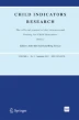
Figures 1 and 2 illustrate the distributions of the direct estimates of childhood development vulnerability at the regional (SA3) level, and plots this against the socioeconomic (IRSD) and remoteness (ARIA) indices respectively. The figures show that there is an explicit negative and positive relationship of the regional prevalence of vulnerability with the corresponding relative advantage and the remoteness of the area respectively.

Fig. 1

Prevalence of Childhood Vulnerability in Physical Health and Wellbeing in each SA3 region (with socio-economic disadvantage and the proportion of Indigenous people in a region). Selected regions of interest are highlighted. The red line shows the linear relationship between Vulnerability with socio-economic disadvantage (IRSD) (continuous) is shown. On the right panel, IRSD scores are discretised

Fig. 2

Prevalence of childhood vulnerability in Physical Health and Wellbeing in each SA3 region (with remoteness/accessibility and the proportion of Indigenous people in a region). Selected regions of interest are highlighted. The red line shows the linear relationship between Vulnerability with remoteness (ARIA) scores (continuous) is shown. On the right panel, ARIA scores are discretised

There is a well established relationship between Indigeneity and socio-economic disadvantage (see for example, Biddle (2014), Biddle and Yap (2010), Jorm et al. (2012); SCRGSP (2011)) and and also between remoteness and Indigenous status (see for example, Thurber et al., 2015). In the main, regions with higher ARIA scores (i.e., more remote and isolated) tend to have larger Indigenous populations. Additionally, since Indigenous people experience more disadvantage, areas with lower IRSD scores (i.e., relatively disadvantaged) tend to have a higher proportion of Indigenous people. In both Figs. 1 and 2, we add a third dimension, the proportion of Indigenous people in the region, captured through the bubble size which reveals nuance to the relationship between socio-economic advantage and remoteness with child developmental vulnerability. The figures reveal that, in general, regions with larger proportions of Indigenous people tend to be both remote and also socio-economically disadvantaged, and in turn have higher levels of child developmental vulnerability.

We draw attention to nine regions, whose names have been superimposed in Figs. 1 and 2. These are the four areas that tend to appear in the top of the graphs - Barkly, Katherine, East Arnhem and Daly-Tiwi-West Arnhem (all located in the Northern Territory). We also highlight five other regions - Hervey Bay (in Queensland), Devonport (in Tasmania), Manly (in New South Wales), Playford and Adelaide City (both in South Australia). These have been selected because they highlight the spatial variation, provide valuable insights, and demonstrate the importance of model-based estimation in improving the available estimates required for policy and planning.

Barkly is located in Central Australia and has a population of roughly 8,000 people on area of 303,000 square kilometres (approximately the size of the United Kingdom). 65% of the population identify as Aboriginal and/or Torres Strait Islanders, and the region is made up of small town-based and remote communities separated by long distances. The living conditions in these communities are generally poorer and have limited opportunities compared to other areas in Australia with better access to jobs, training, education, investment and services, and as such are more vulnerable.

Katherine is located south of Darwin, with a population of roughly 25,000, of which 60% identify as Aboriginal and/or Torres Strait Islanders. Half the regional population are resident in the regional centre, also named Katherine, which has the highest rates of homelessness and overcrowding in Australia. The town and region face profound health and social inequities with a recent report showing that residents live on average 15 years less than the national average (Quilty et al., 2019).

East Arnhem is situated in the far north eastern corner of the Northern Territory. The area is home to approximately 11,000 people living nine major remote communities (five of them located on islands) and other smaller outstations and homeland scattered throughout the region. Over 90% of the population identify as Aboriginal and Torres Strait Islanders (ABS, 2016d).

Daly-Tiwi-West Arnhem is a large remote area with a population of roughly 19,000 people in widely dispersed communities (two on the Tiwi Islands). Approximately three quarters of the population identify as identify as Aboriginal and Torres Strait Islanders. While the general population structure of the Northern Territory shows a marked difference to the Australian average, with higher proportions of children and young adults, and lower proportions of elderly people aged 60 years and above, the Daly-Tiwi-West Arnhem population follows a similar overall trend to the Northern Territory. However, it has an even higher proportion of children: 1 in 5 of the population are children aged under 10 years old (ABS, 2016c; PHNNT, 2020).

The Hervey Bay region is a popular destination for migrants due to the lifestyle advantages offered by its coastal areas due to its favourable climate, relative housing affordability and its proximity to Brisbane, the state capital. However this is mainly concentrated in the northern coastal suburbs, resulting in a rapidly aging population with a privileged socio-economic status. In the surrounding seaside villages and urban settlements, such as Urangan, Aldershot and Eli Waters, the population is younger, more socio-economically disadvantaged, and with a larger Aboriginal and Torres Strait islander population (ABS, 2016e).

Approximately 60% of the Tasmanian population live outside the state capital of Hobart - in contrast, 25% of people in New South Wales live outside Sydney. Devonport is unique in being a regional city and its relative isolation creates challenges associated with a dispersed population such as service provision, access to health and social exclusion. It is characterised by an aging population as a result of elderly retirement migration which is compounded by young people leaving the region.

Playford is located in the northern suburbs of Adelaide, but regularly ranks amongst the most disadvantaged areas in South Australia. Playford has the highest number of people who identified as Aboriginal and/or Torres Strait Islander in South Australia, although the remote areas in the far north (Anangu Pitjantjatjara Yunkunytjatjara) which has the largest proportion (almost 90%) of people who identified as Aboriginal and/or Torres Strait Islander. In contrast, the Adelaide City region, covers the central business district, with a mix of commercial, cultural and entertainment premises and low density housing. The population is dominated by socio-economically advantaged, young, 20-30 year olds, with a relatively low proportion of children (approximately 5% of the population are children under 14 years old) (ABS, 2016g).

Finally, Manly is a beachside area located in northern Sydney. It is relatively affluent with real estate prices amongst the highest in Australia. The area is fairly densely populated with a population size of around 45,000 people, of which 15% are children under 14 years old (ABS, 2016f).

In this section, we compare the results obtained from the fitted models in terms of unbiasedness and consistency as well as the above mentioned discrepancy measures. The different small area estimates of prevalence produced by the models Eq. 3 are subject to uncertainty, but ultimately we want to choose the best performing model based on its (a) consistency with the direct estimate, (b) improved precision (smaller uncertainty), and (c) the interpretability and reasonableness of the estimates in terms of an improved understanding of the phenomenon being studied. We also place these results in context through showing how our model performs in respect to the nine regions (which were selected to cover the different areas with economic (dis)advantage and remoteness/accessibility) discussed above.

Since the two model covariates - socio-economic disadvantage and remoteness/accessibility are significantly associated with the spatial patterns of childhood vulnerability at the regional level, in the model selection we have to choose the best model which does not tend to over- or under-smooth. An over-smoothed model will distort genuine deviations in the data (Smith et al., 2015) while an under-smoothed model can lead to large prediction errors and biased hypothesis tests (Peng et al., 2006).

By definition, ARIA values of zero signify ‘perfect’ accessibility, and that individuals resident in these populated localities do not need to travel significant distances to access services. All major cities (i.e., 160 out of 333 SA3s) are considered to be highly accessible, and as such have zero values. Modelling continuous variables where roughly half of the observations are zero causes problems, and can show non-linearity, which may in turn invalidate the modelling assumptions. This non-linearity is shown in Fig. 2 (left-panel), although not significant. To ameliorate this, we use the discretised version of remoteness, RA (with major cities (160), inner regional (79), outer regional (61), remote (14), very remote (19)). This distinctly shows the linear relationship more clearly in right-panel of Fig. 2. However, discretising the socio-economic disadvantage score (IRSD) into quintiles or deciles is not entirely appropriate, in our case. There is an obvious monotonous relationship between IRSD and vulnerability. But this relationship is not so apparent for the discretised version (see right-panel of Fig. 1). Additionally, while the continuous version pertains to only one covariate, the discrete version pertian to either five (quintiles) or ten (deciles), which increases the number of parameters in the model and is not considered to be efficient.

4.3 Improvement of Estimates

In the results presented here, for demonstrative and brevity purposes, we focus this discussion on one domain: physical health and wellbeing. Similar patterns were found in the other domains. (The rest of the results are in the file provided).

First, the prevalence of child development vulnerability at the state and territory level estimated by the direct and model-based estimators M0 to M4 were compared. Second, we examined the performance at different levels of remoteness (i.e., major cities, regional and remote), to show which estimator was best able to capture the spatial variability in the prevalence of vulnerability.

The comparison of different estimators at state and territory level shown in Fig. 3 indicates that M0 and M1 model-based estimators provide biased estimates for the NT and ACT territories, while M2 and M3 model-based estimators provide biased estimates for all the state and territories except NSW, VIC, and WA. The inclusion of state variable in model M4 overcomes the issues of biasedness for all the states and territories.

Fig. 3

State and territory level prevalence of child development vulnerability in Physical Health and Wellbeing estimated by the model-based estimators M0 to M4 along with the direct estimator (DIR)

To understand how the model-based estimators perform at the state, SA4 and SA3 level, and different remoteness classifications, we examined the bias and mean error as a way of comparing between the estimators. The mean value of relative bias (RB, %) and absolute relative bias (ARB, %) are shown in Table 3, which indicate, on the one hand, that the model M4 provides best performance at the state and territory level, the model M3 at the SA4 level, the model M2 at the SA3 level due to accounting for the respective level-specific variations. Since model M2 takes account of remoteness and SA3 level variability, it provides smallest ARB when compared to the model-based estimators by remoteness of SA3 domains. It is noted that the values of ARB increase with the increase of remoteness. When SA4 level random effects and state level fixed effects are added consecutively in model M3 and M4, the ARB increased due to benchmark the SA3 level estimates with the higher aggregation levels. The considered model M4 provides the least mean value of RB and ARB at the state and territory level. Thus the M4 model-based estimates at SA3, SA4 and state level are numerically consistent from the bottom-to-top administrative hierarchies by accounting for the all the level-specific variations.

Table 3 Mean of relative bias (RB, %), absolute relative bias (ARB, %) relative reduction of standard error (RRSE, %) and CV ratio (%) for the M0 to M4 model-based estimators by state and territory, SA4, SA3 levels as well as the remoteness of SA3 level regions

Furthermore, the models with spatial effects M0 and M1 are directly comparable to M4, which shows very similar performance except at the State level due to bias estimates for ACT and NT (shown in Fig. 3). However, the mean value of ARB is found smaller in model M4 compared to models M1 and M0 for the SA3 domains by their remoteness status shown in Table 3, particularly in remote and very remote SA3 domains. These showed that model M4 provides comparatively better performance.

To compare the model-based estimators in terms of accuracy, the estimated standard errors were compared with the corresponding direct standard errors. We find that at the state level, on the one hand, model M0 and M1 provided very similar levels of accuracy as the direct estimates for all the states except NT and ACT (relatively smaller in populations). On the other hand, M4 provides similar levels of accuracy to the direct estimator for all states/territories. Additionally, M2 and M3 model-based estimators performed poorly with smaller standard errors for most of the states. Note that both these models do not specifically include terms to capture the SA4 and state level variations. However, all the model-based estimators perform better than the direct estimator as expected at the SA4 and SA3 levels.

The obvious differences between model M1 (with spatial effects) and M4 (without spatial effects) is more apparent for the domains with less accuracy, i.e., higher standard errors of direct estimates. These domains with inaccurate (in terms of standard error) direct estimates are primarily found in the remote and very remote areas. We find that model M1 provides higher accuracy (lower standard error), while model M4 provides less accuracy (higher standard error). This shows the pitfalls of simply relying on smaller standard errors to choose between competing small area models. M1 does not account for the remoteness information, as well as the state level variation, while model M4 does, and is preferable, since it better captures the characteristics of the remote (and very remote) domains, which have been shown to have greater levels of vulnerability.

The average values of RRSE indicate that models M2, M3 and M4 provide higher RRSE (i.e., higher standard error) at SA3, SA4 and state levels respectively, due to accounting for corresponding level-specific heterogeneity. Moreover, model M4 provides standard errors closer to the direct estimates at the state/territory level. (We tend to believe these state/territory estimates as ‘ground truth’ due to having a larger number of children at that level.) But model M4 has the added benefit of improving the accuracy at both SA4 and SA3 level reflected by higher RRSE values. This pattern is also true when the performances are compared by remoteness of SA3 domains. The CV ratio for model-based estimators to the direct estimator also confirms that the model M4 performs very well, when contrasted with the direct estimator at the state level. M4 also outperforms the other model-based estimators at the SA4 and SA3 levels. While the spatial models M0 and M1 exhibit similar behaviour at SA3 and SA4 level, they provide biased estimates with higher accuracy at the sate level. On the other hand, the distributions of ARB and RRSE (as well as CV ratio) at SA3 level by remoteness confirm that the model-based estimator M1 provides biased estimates with higher accuracy. In contrast, M4 provides unbiased estimates with slightly less accuracy. This is the trade off between bias and accuracy for the M4 model-based estimator in case of remote and very remote SA3 domains.

In other words, the spatial and non-spatial models provide very similar performance in non-remote areas (Major cities, inner and outer regional), in terms of bias and accuracy, while the non-spatial model (M4) provides less biased estimates with slightly higher standard error as expected due to higher uncertainty in the remote and very remote areas.

4.4 Performance of Model-based Estimators Under Specified Cases

To examine why model M1 with spatial effects performs poorly even after inclusion of the remoteness variable, the bias estimates corresponding to M0, M1 and M2 (red, green and blues circles, respectively) are plotted against the rank of SA3 domains as per IRSD score, ARIA score and the proportion of Indigenous adults in Fig. 4 for the inner and outer regional, remote and very remote SA3 domains. At first appearance, it seems most of blue circles tend to lie close to the zero horizontal line, compared to the others in either case of remote and very remote areas (first column) or inner and outer regional areas (second column). On closer inspection, however, it can be seen that the scatter plots under the first column show that the differences between M0 and M1 models are comparatively small compared to the difference between M0 and M2 models for most of the domains where IRSD score is lower, and ARIA score as well as the Indigenous proportion are comparatively higher. Similar patterns are observed for inner and outer regional areas but the difference is less pronounced. This means that spatial model M1 failed to account the remoteness characteristics due to spatial effects, while non-spatial model M2 succeeded to capture the remoteness information and provides more unbiased estimates in remote and very remote areas. A similar investigation among M2, M3 and M4 shows minimal difference in the bias, which are mainly due to adjustment for SA4 and state level variations (figure not shown).

Fig. 4

Difference in bias among the models M0, M1 and M2 to distinguish how the SA3 level spatial effects fail to understand the effect of remoteness of the SA3 domains on the child development vulnerability in physical health and wellbeing. Comparatively Model M2 provides better performance overall

The comparison of the model-based estimators for the considered specific SA3 areas is shown in Fig. 5, which indicates that the model M4 perform explicitly better than M0 and M1 for the very remote SA3 regions, such as Barkly, and Katherine in NT. This figure also shows that model M4 provides more consistent estimates, and better accounts for regional and socio-economic associations in the prevalence of child vulnerability.

Fig. 5

SA3 level prevalence of child development vulnerability in physical health and wellbeing estimated by the model-based estimators M0 to M4 along with the direct estimator (DIR) for some unique regions

These detailed comparisons of the models for the specified locations, show the importance of adjusting for the remoteness of the regions (i.e., models M3 and M4) instead of specifically accounting for spatial effects ignoring the remoteness characteristics (i.e., models M0 and M1). These differences are not entirely apparent when examining the model fit and model performance statistics – in the main because there is relatively little to compare between the direct and the various model-based estimators, on average. But the relative utility of including socio-economic disadvantage and remoteness in understanding the spatial variability is more apparent in remote and very remote regions.

In summary, we can see that the model with SA3 level spatial effects fails to smooth the direct estimates correctly, since the model can not adequately capture the effect of remoteness on the vulnerability of childhood. This is more apparent when considering model M1. The model fails to distinguish the geographical correlation between neighbouring regions from the effect of remoteness and accessibility. Subsequently, the smoothing leads to biased and inefficient inference for the remote and non-remote neighbouring regions.

Fig. 6

Graphical posterior predictive checks evaluate the prevalence of child development vulnerabilities in Physical Health and Well-being, as estimated by model-based estimators M0 and M4 across SA3, SA4, and state and territory levels. The black line depicts the distribution of the observed outcomes and lighter lines illustrate the kernel density estimates derived from the posterior predictive distributions

5 Conclusion

There is remarkable geographical variation in the prevalence of childhood vulnerability and this is associated with socio-economic disadvantage and remoteness/accessibility, particularly in Australian communities. As a measure of spatial disadvantage in Australia, using the relative isolation of areas (through the remoteness/accessbility index) combined with the area’s level of socio-economic disadvantage (through the socio-economic index) provides a very useful indication of the socio-spatial determinants of different phenomena. Our work using data from AEDC found that the modelled prevalence in vulnerability was lower in major cities and more wealthier areas, but was higher in less affluent and more remote regions. Our model covariates of socio-economic disadvantage and remoteness/accessibility were significantly associated with the spatial patterns of childhood vulnerability at the regional level. We found that remoteness/accessibility is better captured in discrete form (i.e., with five categories of major cities, inner regional, outer regional, remote and very remote).

The covariate effects account for the spatial patterns due to areas that are socio-economically similar and have similar levels of relative isolation tending to have similar values of child vulnerability. This ‘similarity’ can be used to ‘borrow strength’ over neighbouring areas to obtain more reliable area-specific estimates. In the Bayesian model we combine the prior knowledge about the intrinsic behaviour of spatially related data, and this spatial structure is specified with a set of spatially autocorrelated random effects, in addition to the potentially available covariate information, through spatial smoothing.

Spatial smoothing has the benefit of more appropriately representing the statistical uncertainty of the model parameters, giving better predictions, and providing greater insights into the observed associations in data, and their underlying mechanisms (Duncan & Mengersen, 2020). However, spatial smoothing accounts for spatial correlation through relying on neighbouring regions (areas) - this is a direct result of Tobler’s First Law, which states that ‘near things are more related than distant things’ (Tobler, 1970). In our study, on the one hand, we showed that the spatial and non-spatial models provide very similar performance in the non-remote areas (Major cities, inner and outer regional), in terms of bias and accuracy. On the other hand, the non-spatial model provides more reasonable estimates in the remote and very remote areas.

In Australia, where the population is sparsely spread out, spatial smoothing can be problematic. We find that there are considerable differences in the smoothing properties of the spatial effects - particularly, in areas of relative affluence or deprivation, or relative remoteness/isolation when compared with neighbouring areas. In these instances, including the model covariates - here, socio-economic disadvantage and remoteness/accessibility - appear to sufficiently capture the spatial patterns adequately. Any remaining differences are much better captured by specifying a random effect term (due to the unobserved differences in the patterned behaviour of child vulnerability). Including the state term in the model of ensuring consistency between the direct and model-based estimates.

Our results need to be taken with caution. First, there are limitations of using SEIFA and ARIA indices which are designed to reflect area-based attributes, and not individual circumstances. Additionally we are studying characteristics of children (i.e., child vulnerability), but using adult socio-economic and geographical adult characteristics. However, these have been shown to be inextricably linked (Brooks-Gunn & Duncan, 1977). Second, while the models result in improved regional estimates of developmental vulnerability, particularly in areas that are both socio-economically disadvantaged and (geographically) isolated, the models do not capture the spatial disadvantage in major cities. Second, unlike other small area problems, the direct estimates are fairly accurate mainly because the participation in the AEDC sample is relatively high (the overall participation over the different cycles averages around 97%) (DET, 2019). As a result, there are not substantive differences between the model-based estimates and direct survey estimates, although stark differences are exhibited at lower levels of geography. Our current work is extending these models to lower geographical levels, i.e., SA2 or SA1. Finally, adding spatial effects can lead to over-smoothing where genuine deviations in the data are removed, leading to greater uncertainty about the model parameters, poorer predictions and misguided inference (Smith et al., 2015). Nonetheless, disaggregated analysis using only information from the direct estimates is not possible due to the fact that the prevalence of child development is, thankfully, uncommon in the population, and as such model-based estimates using small area estimation provides reliable information which is very valuable for policy planning.

There is substantial evidence that children’s experiences of disadvantage are multi-faceted and complex, and for that reason childhood vulnerability is significantly affected by the socio-economic and geographic circumstances in which children find themselves in OECD (2019). Understanding the spatial variation of childhood vulnerability in a country with unique geographic features as Australia, has significant policy implications, as it highlights the importance of providing targeted support to vulnerable populations and subsequently addressing entrenched inequities. We draw attention to a couple of policies that can be provided. First, targeted interventions such as early childhood education centres have been fundamental in addressing persistent disadvantage in economically disadvantaged communities through leading to better health, education and employment outcomes in later life (Ellenbogen et al., 2017; Zubrick et al., 2022). Second, the results can be used to identify areas for prioritised resource allocation, and initiatives to address disparities in access to healthcare for improved equity (Bull et al., 2022). Finally, increasingly governments are using behavioural modelling to find complex solutions to design strategies and policy levers that can improve the lives of Australians (paid parental leave, increased funding in low-income areas, investment in community infrastructure (such as safer environments)) - reliable data on early childhood vulnerability is often critical in these models (Sollis et al., 2022).

Appendix

Table 4 Summary of number of children participating in AEDC 2018 in each SA3 by (i) State and Territory, and (ii) Remoteness

References

Abascal, A., Rothwell, N., Shonowo, A., Thomson, D. R., Elias, P., Elsey, H., & Kuffer, M. (2022). Domains of deprivation framework for map** slums, informal settlements, and other deprived areas in LMICs to improve urban planning and policy: A sco** review. Computers, Environment and Urban Systems, 93, 101770.
ABS. (2001). 1244.0– information paper: ABS views on remoteness, 2001. Australian Bureau of Statistics (ABS). Accessed 11-April-2023
ABS. (2008a). 2039.0 - information paper: An introduction to socio-economic indexes for areas (seifa), 2006. Australian Bureau of Statistics (ABS). Accessed 11-April-2023
ABS (2008b). Regional population. Australian Bureau of Statistics (ABS). Accessed 11-April-2023
ABS (2016a). 1270.0. 55.001– Australian Statistical Geography Standard (ASGS): Volume 1– main structure and greater capital city statistical areas July 2016. Australian Bureau of Statistics (ABS). Accessed 11-April-2023
ABS (2016b). 2033.0.55.001– socio-economic indexes for areas (SEIFA) 2016. Australian Bureau of Statistics (ABS). Accessed 11-April-2023
ABS (2016c). Daly - Tiwi - West Arnhem - 2016 census Aboriginal and/or Torres Strait Islander people quickstats. Australian Bureau of Statistics (ABS), https://www.abs.gov.au/census/find-census-data/quickstats/2016/ IQS70203, Accessed 11-April-2023
ABS (2016d). East Arnhem (R) - 2016 census all persons quickstats. Australian Bureau of Statistics (ABS), https://www.abs.gov.au/census/find-census-data/quickstats/2016/LGA71300, Accessed 11-April-2023
ABS (2016e). Hervey Bay - 2016 census Aboriginal and/or Torres Strait Islander people quickstats. Australian Bureau of Statistics (ABS), https://www.abs.gov.au/census/find-census-data/quickstats/2016/IQS31904, Accessed 11-April-2023
ABS (2016f). Manly - 2016 census Aboriginal and/or Torres Strait Islander people quickstats. Australian Bureau of Statistics (ABS), https://www.abs.gov.au/census/find-census-data/quickstats/2016/IQS12201, Accessed 11-April-2023
ABS (2016g). Playford - 2016 census Aboriginal and/or Torres Strait Islander people quickstats. Australian Bureau of Statistics (ABS), https://www.abs.gov.au/census/find-census-data/quickstats/2016/IQS40202, Accessed 11-April-2023
ABS (2021). Aboriginal and Torres Strait Islander people: Census 2021. Australian Bureau of Statistics (ABS). Accessed 11-April-2023
Adair, T., & Lopez, A. (2020). Widening inequalities in premature mortality in Australia, 2006–16. Australian Population Studies, 4(1), 37–56.
AIHW (2004). Rural, Regional and Remote Health: a Guide to Remoteness Classifications. Australian Institute of Health and Welfare (AIHW), Australian Government. Accessed 11-April-2023
AIHW (2008). Rural and Remote Health. Australian Institute of Health and Welfare (AIHW), Australian Government. Accessed 11-April-2023
AIHW (2015). The Health and Welfare of Australia’s Aboriginal and Torres Strait Islander Peoples: 2015. Australian Institute of Health and Welfare (AIHW), Australian Government. https://doi.org/10.25816/5ebcbd26fa7e4 Accessed 11-April-2023
AIHW (2022a). Aboriginal and Torres Strait Islander Stolen Generations and descendants: numbers, demographic characteristics and selected outcomes. Australian Institute of Health and Welfare (AIHW) Online Report
AIHW (2022b). Indigenous health and wellbeing. Australian Institute Of Health And Welfare (AIHW), Australian Government. https://doi.org/10.25816/5ebcbd26fa7e4 Accessed 11-April-2023
Aizer, A., & Currie, J. (2014). The intergenerational transmission of inequality: Maternal disadvantage and health at birth. Science, 344(6186), 856–861.
Anderson, I., Crengle, S., Kamaka, M. L., Chen, T.-H., Palafox, N., & Jackson-Pulver, L. (2006). Indigenous health in Australia, New Zealand, and the Pacific. The Lancet, 367(9524), 1775–1785.
Anselin, L. (1995). Local indicators of spatial association-lisa. Geographical Analysis, 27(2), 93–115.
Baade, P. D., Turrell, G., & Aitken, J. F. (2011). Geographic remoteness, area-level socioeconomic disadvantage and advanced breast cancer: A cross-sectional, multilevel study. J Epidemiol Community Health, 65(11), 1037–1043.
Badcock, B. (1997). Recently observed polarising tendencies and Australian cities. Australian Geographical Studies, 35(3), 243–259.
Baffour, B., Chandra, H., & Martinez, A. (2019). Localised estimates of dynamics of multi-dimensional disadvantage: An application of the small area estimation technique using Australian survey and census data. International Statistical Review, 87(1), 1–23.
Besag, J. (1974). Spatial interaction and the statistical analysis of lattice systems. Journal of the Royal Statistical Society: Series B (Methodological), 36(2), 192–225.
Biddle, N. (2014). Measuring and analysing the wellbeing of australia’s indigenous population. Social Indicators Research, 116, 713–729.
Biddle, N., & Yap, M. (2010). Demographic and socioeconomic outcomes across the indigenous australian lifecourse: evidence from the 2006 census. CAEPR Research Monograph No 31, Canberra: ANU Press.
Bivoltsis, A., Christian, H., Ambrosini, G. L., Hooper, P., Pulker, C. E., Thornton, L., & Trapp, G. S. (2023). The community food environment and its association with diet, health or weight status in Australia: A systematic review with recommendations for future research. Health Promotion Journal of Australia, 34(2), 328–365.
Boonstra, H.J. (2021). mcmcsae: MCMC Small Area Estimation Computer software manual. R package version 0.7.0
Boonstra, H.J., & van den Brakel, J. (2018). Hierarchical Bayesian time series multilevel models for consistent small area estimates at different frequencies and regional levels. Statistics Netherlands discussion paper, December 4, 2018
Boonstra, H.J., van den Brakel, J., & Das, S. (2021). Multilevel time-series modeling of mobility trends in the Netherlands for small domains. Journal of the Royal Statistical Society: Series A (2)
Brinkman, S. A., Gregory, T. A., Goldfeld, S., Lynch, J. W., & Hardy, M. (2014). Data resource profile: the Australian early development index (AEDI). International Journal of Epidemiology, 43(4), 1089–1096.
Bronfenbrenner, U. (1979). The ecology of human development: experiments by nature and design. Harvard University Press.
Brooks-Gunn, J., & Duncan, G.J. (1997). The effects of poverty on children. The Future of Children, 55–71,
Bull, C., Howie, P., & Callander, E. J. (2022). Inequities in vulnerable children’s access to health services in australia. BMJ Global Health, 7(3), e007961.
Burke, T., & Hulse, K. (2015). Spatial disadvantage: why is Australia different?. Australian Housing and Urban Research Institute. https://www.ahuri.edu.au/research/research-papers/spatial-disadvantagewhy-is-australia-different ISBN 9781922075703
Carter, J., Rutherford, S., & Borkoles, E. (2021). Covid-19 vaccine uptake among younger women in rural Australia. Vaccines, 10(1), 26.
Cheers, B. (1990). Rural disadvantage in Australia. Australian Social Work, 43(1), 5–13.
Collier, L. R., Gregory, T., Harman-Smith, Y., Gialamas, A., & Brinkman, S. A. (2020). Inequalities in child development at school entry: A repeated cross-sectional analysis of the Australian Early Development Census 2009–2018. The Lancet Regional Health-Western Pacific, 4, 100057.
Cramb, S., Duncan, E., Baade, P., & Mengersen, K. (2018). Investigation of Bayesian spatial models. Brisbane: Cancer Council Queensland and Queensland University of Technology (QUT).
Das, S., van den Brakel, J., Boonstra, H. J., & Haslett, S. (2022). Multilevel time series modelling of antenatal care coverage in Bangladesh at disaggregated administrative levels. Survey Methodology, 48(2), 401–437.
DET (2019). Australian Early Development Census National Report 2018. Department of Education and Training (DET), Australian Government. ISSN 2206-284X (Online)
Duncan, E. W., & Mengersen, K. L. (2020). Comparing Bayesian spatial models: Goodness-of-smoothing criteria for assessing under-and over-smoothing. PloS One, 15(5), e0233019.
Ellenbogen, S., Klein, B., & Wekerle, C. (2017). Early childhood education as a resilience intervention for maltreated children. Abuse and Violence Towards Young Children, 82–95,
Exeter, D. J., Zhao, J., Crengle, S., Lee, A., & Browne, M. (2017). The New Zealand indices of multiple deprivation (IMD): a new suite of indicators for social and health research in Aotearoa. New Zealand. PloS One, 12(8), e0181260.
Figari, F. (2012). Cross-national differences in determinants of multiple deprivation in europe. The Journal of Economic Inequality, 10(3), 397–418.
Gabry, J., Simpson, D., Vehtari, A., Betancourt, M., & Gelman, A. (2019). Visualization in Bayesian workflow. Journal of the Royal Statistical Society: Series A (General), 182, 389–402.
Gelman, A., & Rubin, D. (1992). Inference from iterative simulation using multiple sequences. Statistical Science, 7(4), 457–472.
Goldfeld, S., Woolcock, G., Katz, I., Tanton, R., Brinkman, S., & O’Connor, E.,… Giles-Corti, B. (2015). Neighbourhood effects influencing early childhood development: conceptual model and trial measurement methodologies from the kids in communities study. Social Indicators Research, 120, 197–212.
Haslett, S., & Jones, G. (2010). Small-area estimation of poverty: the aid industry standard and its alternatives. Australian & New Zealand Journal of Statistics, 52(4), 341–362.
Hertzman, C., Power, C., Matthews, S., & Manor, O. (2001). Using an interactive framework of society and lifecourse to explain self-rated health in early adulthood. Social Science & Medicine, 53(12), 1575–1585.
Hugo, G. (2007). Space, place, population and census analysis in Australia. Australian Geographer, 38(3), 335–357.
Hugo, G., Bamford, E., & Dunne, L. (1999). Accessibility remoteness index of Australia (ARIA). Department of Health and Aged Care occasional papers series, 6
Hunter, B., & Gregory, R. (1996). An exploration of the relationship between changing inequality of individual, household and regional inequality in Australian cities. Urban Policy Research, 14(3), 171–182.
Janus, M., & Offord, D. R. (2007). Development and psychometric properties of the early development instrument (edi): A measure of children’s school readiness. Canadian Journal of Behavioural Science, 39(1), 1.
Johnson, A. F., Chandra, H., Brown, J., & Padmadas, S. (2010). District-level estimates of institutional births in Ghana: application of small area estimation technique using census and DHS data. Journal of Official Statistics, 26(2), 341–359.
Jordan, H., Roderick, P., & Martin, D. (2004). The index of multiple deprivation 2000 and accessibility effects on health. Journal of Epidemiology & Community Health, 58(3), 250–257.
Jorm, A. F., Bourchier, S. J., Cvetkovski, S., & Stewart, G. (2012). Mental health of Indigenous Australians: a review of findings from community surveys. Medical Journal of Australia, 196(2), 118–121.
Lakhani, H. V., Pillai, S. S., Zehra, M., Sharma, I., & Sodhi, K. (2020). Systematic review of clinical insights into novel coronavirus (covid-19) pandemic: persisting challenges in us rural population. International Journal of Environmental Research and Public Health, 17(12), 4279.
Leasure, D. R., Jochem, W. C., Weber, E. M., Seaman, V., & Tatem, A. J. (2020). National population map** from sparse survey data: A hierarchical Bayesian modeling framework to account for uncertainty. Proceedings of the National Academy of Sciences, 117(39), 24173–24179.
Leventhal, T., & Brooks-Gunn, J. (2000). The neighborhoods they live in: the effects of neighborhood residence on child and adolescent outcomes. Psychological Bulletin, 126 (2), 309,
Li, M., Baffour, B., & Richardson, A. (2020). Bayesian spatial modelling of early childhood development in Australian regions. International Journal of Health Geographics, 19(1), 1–16.
Manley, D., van Ham, M., & Hedman, L. (2020). Inherited and spatial disadvantages: A longitudinal study of early adult neighborhood careers of siblings. Annals of the American Association of Geographers, 110(6), 1670–1689.
Massey, D. S., Rothwell, J., & Domina, T. (2009). The changing bases of segregation in the united states. The Annals of the American Academy of Political and Social Science, 626(1), 74–90.
McLoyd, V. C. (1998). Socioeconomic disadvantage and child development. American Psychologist, 53(2), 185.
Mendez-Luck, C. A., Yu, H., Meng, Y.-Y., Jhawar, M., & Wallace, S. P. (2007). Estimating health conditions for small areas: asthma symptom prevalence for state legislative districts. Health Services Research, 42(6p2), 2389–2409.
Ministry of Education, New Zealand (2022). Isolation index. https://www.education.govt.nz/our-work/changes-in-education/equity-index/faq-isolation-index-changes/ Accessed 11-April-2023
Mollié, A. (1996). Bayesian map** of disease. Markov chain Monte Carlo in Practice, 1, 359–379.
Moran, P. A. (1950). Notes on continuous stochastic phenomena. Biometrika, 37(1/2), 17–23.
Naghavi, M., Abajobir, A. A., Abbafati, C., Abbas, K. M., Abd-Allah, F., Abera, S. F., et al. (2017). Global, regional, and national age-sex specific mortality for 264 causes of death, 1980–2016: a systematic analysis for the global burden of disease study 2016. The Lancet, 390(10100), 1151–1210.
Needham, C., Sacks, G., Orellana, L., Robinson, E., Allender, S., & Strugnell, C. (2020). A systematic review of the australian food retail environment: Characteristics, variation by geographic area, socioeconomic position and associations with diet and obesity. Obesity reviews, 21(2), e12941.
Noble, M., Wright, G., Smith, G., & Dibben, C. (2006). Measuring multiple deprivation at the small-area level. Environment and Planning A, 38(1), 169–185.
OECD (2019). Changing the odds for vulnerable children building opportunities and resilience. OECD Publishing.
Paradies, Y. (2016). Colonisation, racism and Indigenous health. Journal of Population Research, 33(1), 83–96.
Paradies, Y., Ben, J., Denson, N., Elias, A., Priest, N., Pieterse, A., & Gee, G. (2015). Racism as a determinant of health: a systematic review and meta-analysis. PloS One, 10(9), e0138511.
Peng, R. D., Dominici, F., & Louis, T. A. (2006). Model choice in time series studies of air pollution and mortality. Journal of the Royal Statistical Society: Series A (Statistics in Society), 169(2), 179–203.
Pfeffermann, D. (2013). New important developments in small area estimation. Statistical Science, 40–68,
Phillips, B., Daniels, J., Woodward, A., Blakely, T., Taylor, R., & Morrell, S. (2017). Mortality trends in Australian Aboriginal peoples and New Zealand Māori. Population Health Metrics, 15(1), 1–12.
PHNNT (2020). Daly - Tiwi - West Arnhem Region: Data report. Primary Health Network for the Northern Territory (PHNNT), https://www.ntphn.org.au/, Accessed 11-April-2023
Priest, N., Paradies, Y., Stewart, P., & Luke, J. (2011). Racism and health among urban aboriginal young people. BMC Public Health, 11(1), 1–9.
Quilty, S., Wood, L., Scrimgeour, S., Shannon, G., Sherman, E., Lake, B., & Moloney, M. (2019). Addressing profound disadvantages to improve Indigenous health and reduce hospitalisation: a collaborative community program in remote Northern Territory. International Journal of Environmental Research and Public Health, 16(22), 4306.
R Core Team (2015). R: A language and environment for statistical computing Computer software manual. Vienna, Austria. http://www.Rproject.org
Rae, A. (2009). Isolated entities or integrated neighbourhoods? an alternative view of the measurement of deprivation. Urban Studies, 46(9), 1859–1878.
Rao, J., & Molina, I. (2015). Small Area Estimation (2nd ed.). Wiley-Interscience.
Sampson, R.J., Morenoff, J.D., & Earls, F. (1999). Beyond social capital: Spatial dynamics of collective efficacy for children. American Sociological Review, 633–660,
Sampson, R.J., Morenoff, J.D., & Gannon-Rowley, T. (2002). Assessing “neighborhood effects”: Social processes and new directions in research. Annual Review of Sociology, 443–478,
SCRGSP (2011). Overcoming indigenous disadvantage: key indicators,. (2011). Steering Committee for the Review of Government Service Provision (SCRGSP). Canberra, Australian Capital Territory: Productivity Commission.
Smith, T. R., Wakefield, J., & Dobra, A. (2015). Restricted covariance priors with applications in spatial statistics. Bayesian Analysis (Online), 10(4), 965.
Sollis, K., Yap, M., Campbell, P., & Biddle, N. (2022). Conceptualisations of wellbeing and quality of life: A systematic review of participatory studies. World Development, 160, 106073.
Spiegelhalter, D., Best, N., Carlin, B., & van der Linde, A. (2002). Bayesian measures of model complexity and fit. Journal of the Royal Statistical Society B, 64(4), 583–639.
Tanton, R., Dare, M., Brinkman, S., Corti, B.-G., Katz, I., Woolcock, G., & Goldfeld, S. (2017). Identifying off-diagonal communities using the Australian Early Development Census results. Social Indicators Research, 132, 977–992.
Tanton, R., Gong, C. H., & Harding, A. (2012). Evidence of multiple life stage disadvantage for small areas in Australia. Economic Papers: A Journal of Applied Economics and Policy, 31(1), 76–86.
Thurber, K. A., Banks, E., & Banwell, C. (2015). Cohort profile: Footprints in Time, the Australian Longitudinal Study of Indigenous Children. International Journal of Epidemiology, 44(3), 789–800.
Timms, D. (1971). The urban mosaic: Towards a theory of residential differentiation (No. 2). CUP Archive.
Tobler, W. R. (1970). A computer movie simulating urban growth in the Detroit region. Economic Geography, 46(sup1), 234–240.
Townsend, P. (1979). Poverty in the United Kingdom: A survey of household resources and standards of living. Univ of California Press.
Turrell, G., Kavanagh, A., & Subramanian, S. (2006). Area variation in mortality in Tasmania (Australia): The contributions of socioeconomic disadvantage, social capital and geographic remoteness. Health & Place, 12(3), 291–305.
Van Ham, M., Hedman, L., Manley, D., Coulter, R., & Östh, J. (2014). Intergenerational transmission of neighbourhood poverty: An analysis of neighbourhood histories of individuals. Transactions of the Institute of British Geographers, 39(3), 402–417.
Vehtari, A., Gabry, J., Magnusson, M., Yao, Y., Bürkner, P.-C., Paananen, T., & Nicenboim, B. (2022). loo: Efficient Leave-One-Out Cross-Validation and WAIC for Bayesian Models Computer software manual. R package version 2.5.1
Vehtari, A., Gelman, A., & Gabry, J. (2017). Practical Bayesian model evaluation using leave-one-out cross-validation andWAIC. Statistics and Computing, 27(5), s1413-1432.
Vera-Toscano, E. (2020). The mechanisms underlying the intergenerational transmission of disadvantage: Three examples from australia. Australian Economic Review, 53(2), 247–253.
Vos, T., Barker, B., Begg, S., Stanley, L., & Lopez, A. D. (2009). Burden of disease and injury in Aboriginal and Torres Strait Islander peoples: the Indigenous health gap. International Journal of Epidemiology, 38(2), 470–477.
Wakerman, J., Humphreys, J. S., Wells, R., Kuipers, P., Entwistle, P., & Jones, J. (2008). Primary health care delivery models in rural and remote Australia - a systematic review. BMC Health Services Research, 8(1), 1–10.
Watanabe, S. (2013). A widely applicable Bayesian information criterion. Journal of Machine Learning Research, 14, 867–897.
Whelan, C. T., & Maître, B. (2005). Vulnerability and multiple deprivation perspectives on economic exclusion in Europe: A latent class analysis. European Societies, 7(3), 423–450.
Wilkinson, D., Ryan, P., & Hiller, J. (2001). Variation in mortality rates in Australia: correlation with Indigenous status, remoteness and socio-economic deprivation. Journal of Public Health, 23(1), 74–77.
Wilson, T., Zhao, Y., & Condon, J. (2019). Limited progress in closing the mortality gap for Aboriginal and Torres Strait Islander Australians of the Northern Territory. Australian and New Zealand Journal of Public Health, 43(4), 340–345.
Wilson, W. J. (2012). The truly disadvantaged: The inner city, the underclass, and public policy. University of Chicago Press.
Zubrick, S.R., Taylor, C., Christensen, D., & Hancock, K. (2022). Early years and disadvantage: Matching developmental circumstances in populations to prevention sand intervention opportunities. Family dynamics over the life course: Foundations, turning points and outcomes (pp. 37–56). Springer International Publishing Cham.
Acknowledgements
This work was supported by the Australian National Health and Medical Research Council (NHMRC) under Ideas Grant (APP1184720) ‘Filling in the blanks: a visualisation tool to align national health data with regional health policy objectives’. We wish to acknowledge Australian Government Department of Education for providing access to the statistical area specific Australian EDC 2018 data. We also note that the findings and views reported are those of the authors and should not be attributed to the Department or the Australian Government.
Funding
Open Access funding enabled and organized by CAUL and its Member Institutions.
Author information
Authors and Affiliations
Corresponding author
Ethics declarations
Conflict of interest
None of the authors have a conflict of interest to disclose.
Supplementary Information
Below is the link to the electronic supplementary material.
Appendix
Rights and permissions
Open Access This article is licensed under a Creative Commons Attribution 4.0 International License, which permits use, sharing, adaptation, distribution and reproduction in any medium or format, as long as you give appropriate credit to the original author(s) and the source, provide a link to the Creative Commons licence, and indicate if changes were made. The images or other third party material in this article are included in the article’s Creative Commons licence, unless indicated otherwise in a credit line to the material. If material is not included in the article’s Creative Commons licence and your intended use is not permitted by statutory regulation or exceeds the permitted use, you will need to obtain permission directly from the copyright holder. To view a copy of this licence, visit http://creativecommons.org/licenses/by/4.0/.
About this article
Cite this article
Baffour, B., Das, S., Li, M. et al. The Utility of Socioeconomic and Remoteness Indicators in Understanding the Geographical Variation in the Regional Prevalence of Early Childhood Vulnerability in Australia. Child Ind Res (2024). https://doi.org/10.1007/s12187-024-10143-4
Accepted:
Published:
DOI: https://doi.org/10.1007/s12187-024-10143-4