Astrophotonics: astronomy and modern optics

Abstract

Much of the progress in astronomy has been driven by instrumental developments, from the first telescopes to fiber fed spectrographs. In this review, we describe the field of astrophotonics, a combination of photonics and astronomical instrumentation that is gaining importance in the development of current and future instrumentation. We begin with the science cases that have been identified as possibly benefiting from astrophotonic devices. We then discuss devices, methods and developments in the field along with the advantages they provide. We conclude by describing possible future perspectives in the field and their influence on astronomy.

1 Astronomical instrumentation and science

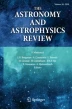
Astronomy is without doubt the empirical science which more than others relies on the analysis of electromagnetic radiation, and as such its progress has often been correlated to the development of optical technology. The most obvious examples of the interaction between science and technology are the discoveries Galileo made at the beginning of the seventeenth century, by pointing his telescope, then the state of the art of optical instrumentation, at the sky. This simple act revolutionized our understanding of the universe, and these early astronomical observations drove the technological developments that allowed science to deliver telescopes of ever-increasing quality. Before the end of the seventeenth century, Christiaan Huyguens was able to develop an aberration-corrected eyepiece allowing him to resolve the rings of Saturn, which were previously believed to be satellites, and detect the rotation of Mars. The invention of the reflecting telescope by Newton, which solved the problem of chromatic aberration, and the development of parabolic mirrors by Gregory ($\sim 1720$), which solved the problem of spherical aberration, opened the possibility to build telescopes with apertures significantly larger than the refractive ones. By the end of the eighteenth century, William Herschel was observing the sky with reflecting telescopes exceeding half a meter in diameter (his largest telescope had an aperture of 122 cm), enabling him to discover faint objects such as the satellites of Saturn and Uranus as well as to compile an extensive catalogue of ‘nebulae’. The invention of the spectroscope by Fraunhofer (1814) and the subsequent discovery of the absorption lines in the spectrum of the Sun is another example of how progress in optical technology eventually changed the course of astronomy. The identification of the spectroscopic signature of chemical elements around 1850 gave astronomers a powerful tool to understand the structure of stars and of the universe, whose benefits we are still exploiting. A visual summary of the progression of optical technology and astronomical discoveries is illustrated in Fig. 1, which shows qualitatively how new technologies, similar to new paradigms, often require about a generation to bring their potential to fulfillment and open new avenues in astronomical discoveries (Kuhn 1962).

Fig. 1

An attempt to compare visually the progress of optics with the discoveries in astronomy. State-of-the-art optical instrumentation has often been the trigger for important discoveries

Today, the frontier in optics is represented by photonics, which is defined as the science dealing with the technologies for generating, transforming or using tailored light states to perform a task. As the word suggests, photonic devices control and manipulate photons in the way electronic devices do with electrons. Using this definition we can include devices such as micro-optics, laser sources, optical filters, optical fibers, and optoelectronic switches, which are commonly used in applications for telecommunications and digital data storage/readout. For this article, we will adopt a more restrictive definition of photonics and will deal mostly with elements requiring the wave approximation of optics to explain properly their operation. Given the impact of optical technologies in sha** the history of astronomy, it is not surprising that astronomers have taken an interest in photonic technologies and potential improvements they could bring to their instruments.

The first examples of what is called now ‘astrophotonics’ (i.e., the application of photonics to astronomical instrumentation Bland-Hawthorn and Kern 2016; Perger et al. 2019).

2.2 Integral field spectroscopy and multi-object spectroscopy: hyperspectral imaging

Whilst spectrographs observing single objects are extremely powerful, they are limited in their capabilities to observe large numbers of objects. In an era where many science cases require large statistical samples and with telescopes becoming fewer in number (due to their larger apertures costing more), more pressures are put on multiplexing, i.e., on the number of objects an instrument can observe at once. Spatial elements (spaxels) are fed from the focal plane into the spectrograph to produce a 3D data cube (see Fig. 3). There are two types of such instruments, which can be loosely classed into MOS and IFS. A MOS allows observations of multiple objects in the field of view (Ellis and Parry 1988) whist an IFS allows small patches of sky to be spatially resolved by an Integral Field Unit (IFU) (e.g., for observation of extended or spatially adjacent objects) (Allington-Smith 2006). To further increase the number and type of object that can be observed there is a combination of the two (using multiple IFUs) which is called Diverse Field Spectrograph (DFS) (Murray and Allington-Smith 2009). There are many science cases for all of the above and some are briefly outlined below.

In a 3D-spectroscopy instrument, the detector plays a central role in determining the final cost (Harris and Allington-Smith 2012), and it is therefore necessary to optimize the use of the detector pixels. Besides the spatial sampling at the telescope, it is necessary to consider the sampling element of the data cube (voxel; Allington-Smith 2006), whose number equals the minimum required number of pixels of the detector. Hence, it is useful to introduce a figure of merit for the instrument, known as specific information density (SID, Allington-Smith 2006):

$$\begin{aligned} \text {SID}=\eta \frac{N_{r}}{N_p}, \end{aligned}$$

(1)

where $\eta$ is the throughput of the instrument, $N_r$ is the number of resolution elements in the datacube and $N_p$ is the total number of pixels of the detector. The relation between the number of resolution elements and spaxels/voxels depends on the type of instrument and should be as close as possible to the maximum value of the SID to improve sensitivity. The SID is maximum when the number of pixels equals the number of voxels and the throughput is one. However, the number of resolution elements is in general smaller than the number of voxels because of oversampling; therefore, the maximum value for the SID will be smaller than 1. In a MOS, one target is sampled by a single spaxel and $N_r=N_sN_{\lambda }/f_{\lambda }$, $N_{\lambda }$ being the number of samples of the wavelength axis, $N_s$ the number of accessible targets, $f_{\lambda }$ being the oversampling factor. If we now assume that there are no unused pixels (condition to maximize SID) the number of voxels will be $N_p=N_s N_{\lambda }$. Taking $f_{\lambda }=2$ (Nyquist sampling of the wavelength), the maximum value for the SID will therefore be 1/2. In an IFS, we will have in general $N_s=N_xN_y$ spaxels (a square array of spaxels is assumed) but the actual spatial resolution elements depend on the oversampling $f_x$ and $f_y$ of the telescope point spread function (PSF) along the coordinates x and y. Thus the number of resolution element is given by $N_r=N_sN_{\lambda }/f_xf_yf_{\lambda }$. With Nyquist sampling in space and frequency, the maximum SID will be 1/8.

Fig. 3

Methods of integral field spectroscopy. The top image shows a lenslet array feeding the spectrograph, this is simple and allows for a large field of view, but requires the spectrograph to be close to the telescope. The second option, fibers, allows the spectrograph to be placed further from the telescope, usually at the cost of throughput. At the bottom, image slicers and microslicers generally allow high throughput, though also require the spectrograph to be close to the telescope. Image reproduced with permission from Allington-Smith (2006), copyright by Elsevier

Galactic science To understand how individual galaxies form, what drives their evolution and what states they tend to, requires large data sets of spatially resolved galaxies. Therefore, large IFSs surveys are an extremely powerful tool. There are currently many large scale surveys such as MASSIVE (Mitchell Spectrograph), AMAZE (SINFONI) and KROSS (KMOS), providing data on hundreds of galaxies. These are being supplemented by even bigger ones (thousands of galaxies observed) such as MaNGA, SAMI, and Califa, plus soon the Local Volume Mapper (LVM). These surveys tend to provide direct information on two components, stars and gas.

New IFSs consisting of several hundred spaxels (e.g. MUSE at the Very Large Telescope (VLT)) are able to access resolved populations of stars in nearby galaxies or globular clusters (Bacon et al. 2010), making detailed kinematic and metallicity studies possible. For more distant galaxies, individual stars cannot be resolved but IFSs can still deliver the radial velocity distribution of their stars, a useful information to identify the morphology of galaxies (Croom et al. 2012).

Studies of the gas in galaxies are equally important. They can be used to trace the metallicity and abundances of the gas, telling us about the processes forming stars and the types of stars that will form and at what rate. In addition, gas can also trace the kinematics of the galaxy.

Combining information on both of these components in large data sets allows astronomers to answer the largest questions in galaxy formation and evolution today. These include how physical processes evolve with time, what regulates star formation, how metals build up, what drives gas inflows and outflows, the role of the local environment and what drives strong morphological transformations.

Cosmology Understanding the universe on the largest scales is one of the grandest aims of astronomy. How the universe expands, the composition of the universe and the physics governing everything are very large questions. To solve these, large sets of data are required. Obtaining these with single slits or fibers is difficult and time consuming. As such the trend is towards MOS instruments. For these surveys, the object is typically not spatially resolved and the science cases are mostly dominated by the desire to understand how galaxies and the corresponding luminosity functions evolve with time.

For this to be known, both the composition and the redshift of the galaxy must be understood. This requires moderate spectral resolving power instruments such as VIMOS (R of 200 to 2500), or AAOmega (R of 1000 to 8000). These instruments are used to perform surveys such as zCOSMOS, VVDS, VIPERS and GAMA. These instruments and surveys have led to many interesting discoveries, such as the combined discovery of periodic variations in the density of visible matter, baryon acoustic oscillations, by the 2dF instrument (Peacock et al. 2001). A current challenge is represented by the observation of faint galaxies with $z\simeq 2$ (the so-called cosmic noon, where star formation had its peak), for which the visible spectrum of their stars appears in the near-infrared. Because of chemo-luminescence generated by the formation of OH radicals in the Earth’s upper atmosphere, spectra of faint galaxies are difficult to acquire and evaluate. This problem has motivated the development of important astrophotonic devices which effectively suppress OH emission lines before a fiber-fed IR spectrograph (see Sect. 4.1).

Direct detection of exoplanets With photometric and time series observations of directly imaged exoplanets we can gain a wealth of information, constraining orbital parameters, size, temperature, surface properties and rotation rate (Traub and Oppenheimer 2010). To perform such observations is challenging, with the planet and star being separated by sub-arcsecond distances with a star-planet contrast of $10^{6}$–$10^{10}$. This means advanced Adaptive Optics (AO) systems are needed, often supplemented by a coronagraph to block light from the star. State-of-the-art systems often employ an additional spectrograph, some with IFU capabilities, such as the IFUs for SPHERE (Claudi et al. 2008), GPI IFU (Chilcote et al. 2012) and CHARIS (SCExAO) (Peters et al. 2012). IFUs not only allow the characterization of the planetary atmosphere (Bowler et al. 2010), but open up the possibility of further reducing contrast using techniques such as spectro-differential imaging (Racine et al. 1999) and molecule map** (Hoeijmakers et al. 2014).

High-angular resolution techniques have been successfully used to push the limit of astrometric precision in the micro-arcsecond range. Examples are some of the major results in the Galactic Center obtained thanks to the sharpest adaptive-optics images of the nuclear star cluster around Sagittarius A$^{*}$ (Schödel et al. 2002; Gillessen et al. 2017; Do et al. 2019) and the recently started 10-$\upmu$as campaign with the GRAVITY interferometer (GRAVITY Collaboration et al. 2017, 2020), which may further change our understanding of strong gravity physics, while building on previous technical progress achieved in the development of astrometric long-baseline interferometers such as PTI (Colavita et al. 1999), PRIMA (Delplancke et al. 2006; Sahlmann et al. 2013) and SIM (Unwin et al. 2008).

2.4 High-contrast techniques

High-contrast science may refer in the first place to the dynamic range of an image, or the amplitude between the readout noise and the saturation limit of the detector. This is particularly an important requirement for the study of stellar clusters, where a compromise between sensitivity and dynamical range needs to be found by adjusting the detector (low/high) gain mode. However, with the rapid expansion in the last decades of the field of exoplanets and planet formation, high-contrast science has developed strong ties to the detection and imaging of faint targets and structures in the immediate vicinity of a bright central source.

Spectacular results in the field of exoplanets and disks have been obtained with the use of coronagraphic instruments capable of significantly reducing the glow of the central star (Oppenheimer and Hinkley 2009). Giant planets have been imaged within 0.5$^{\prime \prime }$ and arcseconds from the their parent A-type stars (e.g.Kalas et al. 2008; Marois et al. 2008; Lagrange et al. 2009) and offer hence excellent prospects for the future spectroscopic characterization of their atmospheres (Janson et al. 2010; Bonnefoy et al. 2016). Spatially resolved sub-structures such as warps and spiral arms have been observed in disks around AU Mic (Boccaletti et al. 2015) and Herbig stars (Benisty et al. 2015) using high-contrast techniques. Very high-precision interferometry in the near-infrared has been successfully employed to characterize the population of debris disks in the Solar neighborhood (Ertel et al. 2014). Beside the existing experience, nulling interferometry may experience a new revival, following the DARWIN/TPF studies (Fridlund 2004; Cockell et al. 2009), for the spectroscopic evidencing of biological biomarkers in the atmosphere of Earth-like planets (Kammerer and Quanz 2018). The recent discovery of a terrestrial, non-transiting, planet orbiting our closest neighbor Proxima Centauri (Anglada-Escudé et al. 2016) will certainly further motivate rapid advances in the field of high-contrast techniques.

Concerning the instrumental requirements applying to high-contrast techniques, the wavefront phase needs to be controlled as well as, or even more stringently than, for imaging or classical long-baseline interferometry. Since contrasts from $10^{-3}$ to $10^{-9}$ need to be achieved, effects related to imperfect Strehl ratios, control of pupil rotation, PSF centering, surface scattering, local intensity mismatches, differential polarization and long-term stability need to be addressed to achieve small inner-working angles (IWA) (Mawet et al. 2012) or deep and stable nulls (Mennesson et al. 2014a). For science cases relevant to exoplanets and planet formation, the requirement of observing in the thermal infrared (L to N, Q astronomical bands) is of high relevance since here the flux contrast between the central star and the planet/disk is more favorable than in the near-infrared or in the optical regimes. Considerations on the spectral richness of infrared spectra in terms of dust & gas tracers and bio-signatures is a further motivation to operate at longer wavelengths. While a high total throughput is desirable to be sensitive to the faintest objects, the possibility to observe in broadband conditions is of high importance as well.

2.5 Metrology and calibration techniques

While not strictly related to one specific science case in astrophysics, the techniques employed for calibration and metrology in support of ground- or space-based observations are indispensible for an optimal interpretation of the science data.

One approach, definable as a passive calibration and likely the most used, consists in observing an astrophysical standard with exactly the same instrumental setup as the one adopted for the science target to identify features extrinsic to the object of interest and calibrate them out. The correction of strong telluric features in spectroscopy, the measurement of photometric standard stars for photometry, and the acquisition of so-called PSF reference stars for spatially resolved imaging are common examples of passive calibration.

Beside this, it is also common to use active calibration systems when a precise knowledge of the time-dependent long-term drifts and stability/uniformity is required, which may be difficult to monitor with on-sky calibration. A good example is high-resolution spectroscopy with a typical resolving power of $R \simeq$100,000 when precise radial velocity measurements are sought for the detection of planets. Since the relative spectral shift of the stellar lines must be determined to a precision on the order of m/s, meaning a precision of $\sim$1/1000 resolution element, high-stability calibration sources such as Thorium-Argon lamps or iodine cells have been employed to track instrumental drifts. While spectral lamps have been central for the operation of the HARPS optical spectrograph, the ESPRESSO spectrograph at the VLT will make use of spectral templates of superior stability and accuracy delivered by a laser frequency-comb Pepe et al. (2010). Artificial sources are also employed to assess the spatial flatness of a detector response, or the quality of the sky thermal background suppression at infrared wavelengths. In wide-field imaging applications, static and dynamic field distortion effects need to be traced, which is typically achieved using an artificial scene of widely and uniformly distributed point sources. Finally, the effective suppression of unwanted sky lines at optical and near-infrared wavelengths by means of carefully tailored narrow-line filters is also highly desirable.

Metrology becomes critical when unavoidable drifts and flexures of a large facility or instrument hamper the ultimate expected accuracy. Mechanical movements can be traced with high accuracy using interferometric methods with a stable, narrow line laser source. For instance, a Helium-Neon laser metrology can achieve (sub-)wavelength position accuracy at 633 nm with an intrinsic relative precision better than 2$\cdot 10^{-9}$. Some application cases can be mentioned: the laser metrology system of the high-precision astrometry instrument Gravity/VLTI launches its 1.9 ${\text{mu}}$m laser beam from the interferometric lab up to the telescope pupil to trace back the path of the astrophysical beam (Lippa et al. 2016). Considering that the astrometric angle $\varDelta \alpha$=$\varDelta$OPD/$B_{p}$, the uncertainty on the length of the projected baseline needs to be sufficiently small not to dominate the overall error budget. With a laser metrology, the precision on the length of the interferometric (projected) baseline $B_{p}$ greatly surpasses what is typically delivered by pointing models; another example of critical metrology need is found with the NEAT (now Theia) project of space-based high-precision astrometric mission (Malbet et al. 2012; Theia Collaboration et al. 2017). The small differential displacement of an Earth-hosting star with respect to the background reference stars due to the orbiting planet can only be measured if the uncertainties on the geometry of the focal plane array (FPA) are calibrated to sub-microarcsecond over many arcminutes (a precision below $10^{-5}$ pixels). An interferometric laser metrology system illuminating the FPA can help to retrieve the position of the PSF centroid (Crouzier et al. 2016).

The instrumental requirements inherent in active calibration and metrology are clearly driven by an excellent knowledge and understanding of the implemented hardware: this means that particular care needs to be taken to study the spectral content, stability and repeatability of a calibration lamp. Modern laser sources have made enormous progress in that respect. The characterization of the transparency range, optical quality and modal content of any passive component involved in the calibration chain (e.g. filters, optical fibers, phase modulators) must result from dedicated lab testing and, ideally, rely on high-TRL devices. Finally, the possibility to simplify the optical design of any calibration or metrology system for stability should be considered as an important requirement: in this sense, optical fibers that can efficiently transport, filter or mix light from different physical locations will play an increasingly important role in astronomical instrumentation.

3 A very short introduction to photonics

In this review, we present astrophotonic instrumentation not only according to their astronomical use, but also from the perspective of the employed photonic technologies. To this end, we use this chapter to introduce basic photonic concepts, such as waveguides and optical modes. These concepts will be used in Sect. 4 to classify astrophotonic instruments and discuss their properties.

Photonic components can be broadly divided into passive and active devices. Passive devices are optical elements introducing a static modification to the properties of light. In these devices, the light power is preserved or, more often, is reduced by losses. In contrast, active devices can dynamically modify the state of light by means of an interaction with an external agent. The output light power in active devices can be greater than its input, the gain being supplied by an external power source (e.g. electricity). As mentioned, in this review we will discuss photonic applications to astronomy based on components modifying the properties of light on spatial scales of the order of the wavelength of light. Under this classification, we can include micro-optics, phase masks such as gratings (see Sect. 4.1), or vortex phase masks (see Sect. 4.4) but not conventional lenses, which do not require the structuring of an optical surface at the micro–nano-scale.

A fundamental component falling in our classification of passive photonic devices is the optical waveguide. This is an heterogeneous optical medium consisting of a region of space with high aspect ratio (the core) characterized by a refractive index higher than its surroundings (the cladding) and transverse dimensions comparable to the wavelength of light. In such a medium, light can be confined in the core and propagate along the long axis (or longitudinal axis, conventionally oriented to coincide with the z-coordinate axis) thanks to the phenomenon of total internal reflection. The physical principle underlying waveguiding can be exemplified by simple considerations in the frame of the geometrical optics approximation. Neglecting light interference effects, we can show that light can propagate in the core of the waveguide if the external divergence angle of light (with respect to the longitudinal axis) is smaller than the numerical aperture of the waveguide:

$$\begin{aligned} NA=\sqrt{n_{\mathrm{co}}^2-n_{\mathrm{cl}}^2}, \end{aligned}$$

(2)

with $n_{\mathrm{co}}$ and $n_{\mathrm{cl}}$ being the refractive indices of the core and the cladding, respectively. The exact modeling of waveguides with transverse core dimensions comparable with the wavelength of light requires the solution of wave-equations and the introduction of the concept of spatial modes, as outlined below.

Optical waveguides can come in the form of a glass fiber or as an element of an integrated optical circuit, i.e., waveguides manufactured on a glass substrate. The state of light in waveguides can be manipulated by means of more complex passive components analogous to macroscopic devices, such as beam splitters (optical couplers), mirrors (Bragg gratings and micro-resonators) or phase plates (birefringent waveguides).

As active devices of interest for astrophotonics, we will consider mainly lasers and phase modulators. Lasers are optical media in which the population of electrons of a radiative electronic transition is inverted with respect to the state of thermal equilibrium. The population inversion is typically obtained by injecting power in the medium as optical radiation or electrical current. Light resonant to a radiative transition in an inverted medium is amplified coherently because of the occurrence of stimulated light emission. Lasing media are typically placed in an optical resonator, where light can be amplified by many orders of magnitude by passing repeatedly in the amplifier thanks to multiple reflection in the resonator. The laser resonator can be fabricated within a single optical fiber or waveguide using FBGs as mirrors, or manufactured in semiconductor waveguides within a laser diode. Photonic phase modulators are devices using an electrical signal to induce a local variation of the refractive index in a waveguide, which can advance or retard the phase of a guided optical field. They are typically based on the electro-optical effect, by which a constant electrical field can alter the birefringence properties of the medium. By including a phase modulator within an integrated Mach–Zehnder interferometer amplitude modulators can be realized as well.

3.1 Optical modes

An important concept in photonics is the optical mode, which is a stationary state (or eigenstate) of an optical system originating from its boundary conditions and the wave nature of light.

Mathematically, modes are solutions of differential equations which describe the physical system under study. Optical modes are solutions of the electromagnetic wave propagation equation:

$$\begin{aligned} \nabla \times \nabla \times \mathbf {E} - \frac{n^2(\mathbf {x})}{c^2}\frac{\partial ^2\mathbf {E}}{\partial t^2}=0, \end{aligned}$$

(3)

which is straightforwardly derived from the Maxwell equations. Here $n(\mathbf {x})$ is the spatially varying refractive index and c is the speed of light. This equation is usually cast into an eigenvalue problem assuming a harmonic dependence in one or more coordinates. As an example, consider the case of the weakly guiding optical waveguide, i.e., a waveguide satisfying the relationship $\varDelta n=n_\mathrm {co}-n_\mathrm {cl}\ll n_\mathrm {cl}$. In this case, we can safely assume that the electromagnetic field is transverse with respect to the axis of the waveguide and that the vectorial components of the electric field are decoupled. This allows writing the wave equation in a scalar form for the amplitude of one of the polarization directions of the field:

$$\begin{aligned} \nabla ^2 E_{x,y}- \frac{n^2(\mathbf {x})}{c^2}\frac{\partial ^2E_{x,y}}{\partial t^2}=0. \end{aligned}$$

(4)

If the refractive index profile of the core is invariant along z, the z-(longitudinal) component of the electric field has a harmonic dependence on time and z:

$$\begin{aligned} E_{x,y}(x,y,z,t)=\psi (x,y)\cdot \exp [i(\beta z - \omega t)] + c.c. . \end{aligned}$$

(5)

As a consequence, the transverse profile of the field $\psi (x,y)$ obeys the following eigenvalue equation, derived by substituting Eq. (5) in the scalar wave equation Eq. (4):

$$\begin{aligned} \left[ \frac{\partial ^2}{\partial x^2} + \frac{\partial ^2}{\partial y^2}+ n(x,y)\frac{\omega ^2}{c^2}\right] \psi =\beta ^2\psi , \end{aligned}$$

(6)

where n(x, y) is now the refractive index distribution in the transverse (x, y) plane, which attains its maximum in the region of the core. If the refractive index distribution has a peak, the eigenvalue equation has a discrete set of solutions, which represent the transverse modes of a waveguide. The eigenvalues are found by imposing everywhere continuity in value and derivative to the field $\psi (x,y)$, a consequence of n(x, y) possessing at most a finite discontinuity in value (Snyder and Love 1983, Chapt. 33). Step index waveguides with circular cross section, i.e., waveguides with a cylindrical core of constant refractive index and abrupt transition to the cladding, are a particular subgroup of waveguides which possess mode profiles in analytical form. They represent a good approximation of real optical fibers, which can support one or more discrete modes, the modal behavior being parametrized by the normalized frequency V:

$$\begin{aligned} V= \frac{2\pi }{\lambda }a\cdot NA, \end{aligned}$$

(7)

where a is the core radius and $\lambda$ the free space wavelength of the light. For V smaller than 2.405, circular waveguides can support only a single mode. Asymptotically the number of modes supported by a step index waveguide with circular cross section is given by:

$$\begin{aligned} N=\frac{V^2}{4}. \end{aligned}$$

(8)

Modes can also have a longitudinal attribute, as is the case of optical resonators, regions of space where light is trapped such as in the volume between two parallel plane mirrors. The mirrors introduce a boundary condition for the electromagnetic field similar to that of a vibrating string (the optical field vanishes at the mirror surface) so that only a discrete set of longitudinal waves characterized by an integer number of half wavelengths are supported by the resonator.

Modes can be excited by matching an external optical field to the modal field distribution at the boundaries of the photonic device. Examples are the excitation of modes in a fiber by illuminating its tip with a beam having the same spatial distribution of the mode or illuminating the semi-reflecting mirror of an optical resonator with light tuned to the frequency of its stationary waves. Modes form a complete orthonormal base for stationary fields sustained by the photonic component and thus their complex amplitude $a_ \mathrm {j}$ can be obtained by projecting the exciting field distribution $E_\mathrm {ext}(x,y)$ onto the mode profile $\psi _\mathrm {j}(x,y)$ at the interface:

$$\begin{aligned} a_\mathrm {j}=\sqrt{\frac{n_{co}}{2}}\left( \frac{\epsilon _0}{\mu _0}\right) ^{1/4}\frac{\int _{S}\psi _\mathrm {j}(x,y) E_\mathrm {ext}^{*}dA}{\left[ \int _{S}\left| \psi _\mathrm {j}(x,y)\right| ^2 dA\right] ^{1/2}}, \end{aligned}$$

(9)

where S represents the external surface of the modal volume. The normalization in this case is chosen so that the power carried by the jth mode is given simply by the square modulus of $a_\mathrm {j}$.

3.2 Modes and seeing

Highly multi-mode fibers can be described safely in the frame of the geometrical optics approximation. This gives us the possibility to use the brightness theorem (Born and Wolf 1997), to describe the seeing limited PSF of a telescope in terms of modes. Moreover, as the brightness theorem is basically a formulation of the second principle of thermodynamics (McMahon 1975), we derive a useful lesson regarding mode transformation devices. The brightness theorem states that the power per unit area and solid angle (the brightness) of the image of a source of light formed by a passive optical system cannot exceed the brightness of the source itself. Since the brightness is related to the temperature of the source, it is clear that a violation of the brightness theorem could allow a perpetual motion machine to work. In a lossless passive optical system the collected power is preserved; thus the brightness theorem is equivalent to stating that the étendue of the source and the image are the same, the étendue ${\mathcal {E}}$ being defined as the product of the source area A and its solid angle divergence $\varOmega$:

$$\begin{aligned} {\mathcal {E}}=A\cdot \varOmega . \end{aligned}$$

(10)

We now consider an optical system consisting of a seeing limited telescope focusing light on a multi-mode optical fiber placed in the focal plane. For the image of starlight in the focal plane of a telescope of diameter $D_{\mathrm{T}}$ and focal ratio $F_\sharp$, the ètendue can be written as

$$\begin{aligned} {\mathcal {E}}_\mathrm {tel}=\pi (\theta D_{\mathrm{T}} F_{\sharp })^2 \pi \left( \frac{1}{2F_\sharp }\right) ^2=\frac{\pi ^2}{4}(\theta D_{\mathrm{T}})^2. \end{aligned}$$

(11)

Here the angle $\theta$ represents the seeing. On the other side, the etendue of light propagating in a step-index optical fiber can be written as the area of the core of radius a by the square of the numerical aperture:

$$\begin{aligned} {\mathcal {E}}_\mathrm {fib}=\pi a^2 \pi NA^2=\frac{V^2}{4}\lambda ^2, \end{aligned}$$

(12)

where we have used the definition of the normalized frequency V of the waveguide Eq. (8). In this case, $\lambda ^2$ can be interpreted as the etendue of a single optical mode. Because in lossless systems the etendue of light is a constant, we can write

$$\begin{aligned} \frac{V^2}{4}\lambda ^2 = \frac{\pi ^2}{4}(\theta D_{\mathrm{T}})^2. \end{aligned}$$

(13)

Recalling that the seeing angle can be roughly defined as $\lambda /r_{\mathrm{0}}$, $r_{\mathrm{0}}$ being the Fried parameter (the correlation length of the atmospheric refractive index distribution; Fried 1966), we obtain

$$\begin{aligned} \frac{V^2}{4} = \frac{\pi ^2}{4}\left( \frac{D_{\mathrm{T}}}{r_0}\right) ^2 \,, \end{aligned}$$

(14)

in which the expression $\frac{\pi ^2}{4}\left( \frac{D_{\mathrm{T}}}{r_0}\right) ^2$ can be interpreted as the ‘modal content’ of the point spread function of the telescope.

The conservation of brightness has further implications which add complexity for astronomical instrumentation. In particular, it shows the impossibility to have a passive, lossless device converting multimode light into a single mode (Welford and Winston 1982). If such a device were possible, the brightness of light confined in the single-mode output should necessarily increase because of the reduction of the\´etendue, thus violating the second principle of thermodynamics. This is the reason why multimode devices with single-mode behavior such as the photonic lantern Leon-Saval et al. (2005); Birks et al. (2015) distribute multi-mode light to an equivalent number of single-mode waveguides.

In active devices, brightness is not preserved, but the corresponding reduction of entropy is compensated by the necessity to extract information from the system. This is for instance the case of an adaptive optics system coupled to a single-mode fiber, which uses the information of the wavefront sensor to correct the wavefront and concentrates the power in a single mode of the fiber. The reduction in entropy associated with the correction of the aberrations is largely compensated by the entropy increase of the wavefront measurement operation, which requires the absorption of light on a detector.

3.3 Spectroscopy

In a simplified dispersive spectrograph, the light enters through a slit that selects a small region of the field, the light is collimated, a prism, grating or other dispersive element disperses the light, and a camera lens focuses the light onto a detection surface. One of the most important requirements for spectroscopy is the achievable spectral resolving power ${R}=\lambda$/$\varDelta \lambda$, which is usually driven by a particular science case. It determines our ability to measure flux densities at two nearby wavelengths separated by $\varDelta \lambda$. For grating spectroscopy, for example, the spectral resolving power is given by

$$\begin{aligned} R = \frac{m \rho \lambda W}{\theta D_{\mathrm{T}}} \,. \end{aligned}$$

(15)

where m is the diffraction grating order, $\rho$ is the ruling density (usually given in lines per mm), $\lambda$ is the operating wavelength, W is the illuminated grating width, $\theta$ is the angular seeing and $D_{\mathrm{T}}$ is the telescope diameter.

This means that in systems where diffraction is dominant ($\theta D_{\mathrm{T}} = \lambda$) the spectral resolving power is limited by the properties of the diffractive element. However, in non-diffraction limited cases ($\theta D_{\mathrm{T}} > \lambda$), R will be constrained by the implemented dispersion element (e.g. grating, prism), the diameter of the telescope feeding it, and the slit size itself. This dependence is well established in classical instrumentation and further information can be found in spectroscopy textbooks (e.g., Schroeder 1987).

3.4 Modal noise

As mentioned in the previous sections, multi-mode fibers contain different modes depending on their properties. Depending on the incident electric field, wavelength, fiber stresses and strains different modes will be excited. With a constantly moving telescope and changing atmosphere, this translates to an ever changing output illumination pattern from the fiber. In an astronomical spectrograph, this phenomenon is known as modal noise and results in a variation of the measured position of the light-spot barycenter on the detector, resulting in a measured wavelength shift.

Whether this variation is important greatly depends on the science case, where wavelength precision is not required this is not a problem; however, for highly precise measurements, e.g. exoplanet detection, this can seriously influence the accuracy of results (Rawson et al. 1980). There are various ways of controlling this, for instance agitating the fiber (Baudrand and Walker 2001) and this works sufficiently for the current generation of spectrographs, which aim for around 1 m/s precision and work in the visible with many modes. However, this problem is particularly pronounced as the number of the modes within the fiber is reduced, statistically increasing the relative uncertainty due to this movement. The next generation of instruments, which will aim for higher precision and those working in the infra-red will be particularly affected.

It must also be noted, that reducing the number of modes to one (not including polarization), eliminates this effect. However, it has been noted that polarization then has a greater effect Halverson et al. (2015).

4 Astrophotonics

In this section, we review photonic devices developed so far for astronomical instrumentation and classify them by astronomical technique and photonic function. As indicated in Fig. 4, we distinguish the six main astronomical techniques (namely spectroscopy, high angular resolution, hyperspectral imaging, high-contrast imaging and metrology/calibration, detection enhancement) whose scope and requirements have been discussed in Sect. 2. The photonic functionality distinguishes three categories depending on the modal content of the key photonic component of the instrument, i.e., single-mode, multi-mode and mode transformation devices. Under single-mode devices, we include continuous wave lasers operating at a single longitudinal mode, or devices based on single-mode optical waveguides. Devices such as laser guide stars and integrated optics beam combiners for interferometry are, therefore, found in this category. Multimode devices are pulsed laser sources, which emit a multitude of longitudinal modes, or devices based on multi-mode optical fibers. Laser frequency combs or 3D spectroscopy instruments (MOS or IFS) are typical representative of this category. In between the single-mode and the multimode categories, we can find mode transformation devices, which modify the modal distribution between input and output. These are for instance passive devices such as the photonic lantern and diffraction gratings (MM to MM), phase masks (SM to SM) or active devices as for example deformable mirrors in an adaptive optical system (MM to SM). The table in Fig. 4 thus gives an overview of the astrophotonic instruments according to the dual classification described above.

Fig. 4

Astrophotonic instruments can be classified according to the scientific purpose (rows) and the modal behavior (columns) of their key photonic component

In the following pages the sub-sections are devoted to the aforementioned astronomical techniques, while paragraphs distinguish the various photonic functionalities underlying the instruments.

4.1 Spectroscopy

Single-mode spectrographs  The mismatch between the diffraction-limited resolution of the telescope $\lambda /D_T$ and the seeing $\theta$ reduces the spectral resolving power of the spectrograph, which can be restored only by making the grating (and hence instrument) larger or reducing the size of the slit (which can cause a loss in light unless techniques such as image slicing are used). The smallest spectrograph is then in general the one for which $\lambda /D_T=\theta$, the so-called diffraction-limited spectrograph. From the point-of-view of astronomical instrumentation, a truly diffraction-limited spectrograph could offer, besides size reduction, two further main advantages. Firstly, improved stability through the elimination of modal noise in fibers (see Sect. 3.4), and second, a further reduction of cost, thanks to either mass-produced components for the photonic market or smaller conventional components.

Astrophotonics aims to create diffraction limited spectrographs by feeding the spectrograph with one or multiple (SMFs) acting as spatial filters (a single-mode spectrograph). Whilst the idea of using spectrographs fed by SMFs is not new to astronomy, coupling starlight to them is notoriously inefficient, due to atmospheric turbulence (Shaklan and Roddier 1988). A sophisticated AO system is therefore still mandatory to reduce coupling losses. Before truly single-mode (SM) coupling was considered, there were attempts using few-mode fibers (FMF) in 1998 (Ge et al. 1998), though with a light loss still unacceptable for astronomical spectroscopy. This restriction means most current spectrographs are fed using multi-mode (MM) fibers. In recent years, developments in extreme adaptive optics (ExAO) systems now routinely allow high Strehl ratios and hence increasingly efficient coupling into SMFs. This is leading to the first generation of SMF fed instrumentation, with examples of coupling tests on SCExAO (Jovanovic et al. 2017b) and full instruments in Minerva-red (Blake et al. 2015) and iLocater (Crepp et al. 2016).

Single-mode reformatters and spectrographs  To overcome the requirement of using ExAO while preserving a high-throughput, single-mode spectrographs fed by a photonic lantern (PL) Leon-Saval et al. (2005); Birks et al. (2015) have been proposed (e.g. the Photonic Integrated Multi-Mode Spectrograph (PIMMS); Bland-Hawthorn et al. 2010). PLs are tapered optical fibers which adiabatically transform a MM optical fiber into a collection of SMFs. Light injected at the MM end of the device is distributed without losses in the output SMFs provided their number is at least equal to the number of modes supported in the MM end. A lossless transition to fewer fibers is in fact prohibited by the brightness theorem (see Sect. 3.2). PLs come in the form of fibers Leon-Saval et al. (2005) or integrated 3D waveguides Thomson et al. (2012); Spaleniak et al. (2013) and can provide single-mode functionality to multi-mode fiber (MMFs). This quality, originally exploited for the development of astronomical notch filters (see below), allows in principle efficient coupling from seeing-limited telescopes, while allowing light dispersion with a compact single-mode spectrograph. The PIMMS concept has two possible implementations, either the SMF ends are rearranged into a linear array acting as the pseudoslit of a spectrograph (also known as reformatting of light), or they are fed to integrated spectrographs (see next paragraph). Further elaborations of the PIMMS concept have been conceived or developed. The simplest is the photonic Tiger concept (named for the fiber fed Tiger IFU Courtes 1982). This means the spectra need to be dispersed such that none of the inputs overlap. Alternatives have been put forward, to use ultrafast laser inscription (ULI) to write a 3D integrated optical component reformatting the multi-core fiber (MCF) into a long slit. These are either separate waveguides (Thomson et al. 2012; Spaleniak et al. 2013) or the waveguides are joined together to form a long slit (MacLachlan et al. 2016a). The advantage of this method is similar to conventional slit techniques, maximizing use of the detector. In addition, fiber reformatters, taking the point spread function (PSF) from the telescope and reformatting into a slit have now been proposed and tested in the lab, showing high levels of throughput (Yerolatsitis et al. 2017). These are efficient, but in their current form limited to low mode counts due to the complexity of the devices.Throughput in low-mode fibers can be improved by improving the PSF of the telescope with a low order AO system (Harris et al. 2015). A preliminary numerical investigation of the trade-off between telescope beam quality and throughput is presented in Diab and Minardi (2018). Some of these devices have been tested on sky either with a spectrograph (e.g. the TIGER spectrograph Leon-Saval et al. 2012), or without (e.g. the Photonic dicer, Harris et al. 2015, and the hybrid reformatter, MacLachlan et al. 2016b).

Integrated photonic spectrographs  As astronomical instruments are constantly growing in size, techniques allowing the reduction of their size and complexity are very popular. In telecommunications, this has been an aim for many years, resulting in the delivery of mature devices on centimeter size scales.

The idea of using these technologies in astronomy was suggested as early as the mid 1990s by Watson (1995, 1997) and was initially based upon Arrayed Waveguide Gratings (AWGs). The AWG works in a similar way to a conventional spectrograph, though embedded within a glass chip, which reduces size and alignment complexity. A sketch of the device is illustrated in Fig. 5. The initial single-mode waveguide can be considered as the slit, or feeding fiber to the spectrograph. The beam diffracts in the first free propagation region, which acts as a collimator thanks to the confocal curved surfaces of its edges (Goodman 2003, Chapt. 4). The expanded beam is sampled by an array of waveguides which, thanks to their curved paths, add a constant incremental phase difference to the light propagating in neighboring waveguides. The output of the array of waveguides is connected to a second free propagation region, this time acting as a camera lens. Similarly to a conventional spectrograph, spectral lines are focused at the curved exit surface of the free propagation region only if the optical path difference from the focus to any pair of outputs of the output array is an integer multiple of the wavelength. In telecommunication applications, single-mode fibers at the output of the second free propagation region are placed at regular intervals to collect the light of separate wavelength-demultiplexed communication channels. Since the incremental optical path difference introduced by the array of waveguides usually corresponds to several optical wavelengths, the AWG operates at high diffraction order ($\sim 25$) like a conventional echelle grating. As a consequence, the free spectral range (FSR) of the AWG is very small, and their use for astronomy requires the introduction of a cross-disperser at its output to separate the diffraction orders.

At the time of Watson (1995) the AWG technology was not considered sufficiently developed to be used for astronomy. During the 2000s, the technology was reconsidered by Bland-Hawthorn and Horton (2006) who compared the AWG and Phased Echelle Grating (PEG) and concluded that the technology was now sufficiently developed for use in astronomy.

Fig. 5

A schematic of an astronomical Arrayed Waveguide Grating (AWG). Here the input is single-mode waveguide, which is fed by light from the telescope. This light passes through the input free propagation zone and enters the waveguide array where a phase difference is added (analogous to a grating). The light is recombined in the output free propagation zone and the spectrum is sampled either at the output of the chip or cross dispersed. Image reproduced with permission from Douglass et al. (2018), copyright by OSA

The first on sky test of a modified commercial AWG was performed at the Australian Astronomical Telescope (AAT), formerly the Anglo-Australian Telescope in Australia (Cvetojevic et al. 2009). For this test the device was coupled to the telescope using a single, SMF. This led to low coupling efficiency with the seeing limited AAT, though high enough to pick up the atmospheric emission lines. As mentioned, due to the designed low FSR ($\approx$ 57 nm) of the device, the IRIS 2 Tinney et al. (2004) spectrograph was used to cross disperse the output to obtain a useful FSR for astronomy. This first prototype displayed a spectral resolving power of around R $\approx$ 2100 in the lab, which was suitable for low-resolution applications (see Sect. 2.1).

In the next set of experiments, various improvements were made (Cvetojevic et al. 2012). These included (1) optimizing production of the devices for efficiency, (2) removing the tapers of the input waveguides in the free propagation zone (FPZ) (which permitted an increased spectral resolving power), and (3) improving the coupling efficiency with the telescope using a PL. A single optimized AWG was then coupled to the IRIS2 spectrometer for cross dispersion.

Recently more efficient devices have focused on improving coupling, either through using a SMF with the extreme AO system SCExAO Jovanovic et al. (2016, 2017). Whilst a high spectral resolving power (of order R = 60,000) AWG Stoll et al. (2017) has been designed, these are more difficult to manufacture and as of writing none have been successfully produced.

Another category of integrated spectrometers proposed for astrophotonic applications is based on the measurement of the temporal coherence of light in a waveguide. The so called Standing Wave Integrated Fourier-Transform Spectrometer (SWIFTS; Le Coarer et al. 2004; and VIMOS; Le Fèvre et al. 2003). This removes the unwanted stars, but it requires accurate manufacture. Re-configurable fiber optic systems now also exist, which increase versatility, such as placement in crowded fields and rearrangement of the fibers to stop resulting spectral overlap on the detector, increasing the efficiency with which the pixels are used (e.g., AAOmega; Sharp et al. 2006 and FMOS; Kimura et al. 2010). This technique also allows the light to be brought to a spectrograph on a stable platform further from the telescope. Whilst this introduces extra optics (such as the addition of a de-rotator at the Nasmyth focus), it means the instrument can remain fixed with respect to the gravity field, increasing stability (Bely 2003). Such instruments are now allowing huge surveys on smaller research grade telescopes (e.g., BOSS Smee et al. 2013). IFS first began in the 1980s (Vanderriest 1980), and it has rapidly expanded to become a mainstay within astronomy. It is achieved through four main methods: image slicers (e.g., GMOS; Dubbeldam et al. 2000; and NIFS; McGregor et al. 2003), lenslet arrays (e.g., SAURON Bacon et al. 2001), fiber slicers (e.g., Allington-Smith et al. 2002) and microslicers (e.g., Content et al. 2013), these are shown and described in Fig. 3. It must be noted that although these all use novel inputs, the spectrograph behind is very similar to the long slit analogue. DFS is also a rapidly expanding field, with instruments such as KMOS (Sharples et al. 2004) and FLAMES (Pasquini et al. 2002) paving the way for instruments planned for the next generation of Extremely Large Telescope (ELT)s (e.g., IRIS; Larkin et al. 2010). Image slicing can also be used to improve the spectral resolution of a spectrograph by reducing the width of the slit (e.g., Avila et al. 2012) and using the technologies developed for MOSs and IFSs allows the output from the telescope to be split into multiple replicated spectrographs (e.g., VIRUS; Hill et al. 2004).

Astrophotonic integral field units  IFUs were first developed in the 1980s. They take a contiguous spatial sample of points and allow spectra to be taken. There are many types of conventional IFU (see Allington-Smith 2006), all with respective advantages and disadvantages.

Recently, multimode astrophotonic IFUs have been proposed in the form of hexabundles. This involves taking multiple MMFs, removing the buffer and reducing the the cladding through etching. These fibers are then arranged into an array and fused together to form a hexabundle IFU. By processing the fibers in this way, the fill fraction (the percentage of light sampled) can be increased. Care must be taken in the process not to cause cross coupling (Bryant et al. 2011), leading to a degradation in the signal.

To date, hexabundles are among the most successful spectroscopic components for astrophotonics. Following on from their initial development, they were used in the SAMI instrument on the AAT (Bryant et al. 2015), which was designed to survey the kinematic structure of galaxies. A future instrument HECTOR is currently planned (Lawrence et al. 2012), as an upgrade to SAMI it will use similar techniques, but with greater and also variable spatial sampling. This allows the cores of galaxies to be better sampled by the fibers.

IFUs consisting of a microlens array coupled to an array of single-mode fibers have also been proposed, to miniaturize astronomical spectrographs. As these are single mode, they would need to be fed by a diffraction limited beam to achieve a high throughput. This means they need either a small telescope, a long wavelength or extremely good AO correction. Currently there are variations in the form of the RHEA (Feger et al. 2014), a MCF fed spectrograph with a microlens glued on-top. Recently using MCFs with 3D printed microlenses on-top used as IFUs to feed diffraction limited spectrographs has also been suggested (Dietrich et al. 2017) and trialed on sky (Haffert et al. 2020).

Large scale IFUs for MOS has also been proposed for large telescopes with PSFs far from the diffraction limit. These would take the PSF from the telescope using highly MM PLs and convert them to few-mode (FM) PLs (Leon-Saval et al. 2017). Whilst the number of fibers would be large, converting down would allow access to SM technologies such as FBGs or ring resonators.

Photonic spectro-interferometry  Spectro-interferometry is the high-angular resolution analogue of 3D spectroscopy,  chromatically dispersing interference fringes to measure the variation of their visibility across the spectrum. If a sufficient number of different telescopes are combined, it is possible to retrieve interferometric images of the target for each wavelength (Millour et al. 2016). Besides the already mentioned 4-telescope combiner for mid infrared (Diener et al. 2017), beam combiners featuring 9 input channels in H-band and active control of the optical path have been developed for aperture masking techniques (Martin et al. 2016) (see next section). As may be evident from the previous text, most of the integrated optics beam combiners were developed in the near-infrared band due to the availability of the very mature silica-based technology, which has been developed for the telecommunication market. However, the astrophysical characterization of a target often requires the analysis of starlight over a wide spectral range, therefore ongoing research in interferometric instrumentation is focusing on devising alternative materials and technologies to extend the spectral coverage of integrated optics beam combiners. In particular, both the booming interest towards cold targets such as debris disks and exoplanets (Kraus and Ireland 2006), where a peak-to-peak attenuation of 0.05 was measured. An improved phase mask was later manufactured (monochromatic attenuation in the lab up to $2\cdot 10^{-3}$) and tested on-sky with a high Strehl, clear aperture, test telescope (diameter 1 inch) (Peters et al. 2008). In the latter experiment, an average attenuation of 3% at visible wavelength (20 nm bandwidth) was attained, most of the contrast loss being attributed to the chromatic dispersion of the phase mask.

An inherent problem of phase masks is indeed that they work only at the design wavelength, as the phase delay introduced by a plate of fixed thickness scales as $\lambda ^{-1}$. This effect can be mitigated by designing a vortex lens composed of two layers made of materials with different dispersive properties (Swartzlander 2005, 2006). The inherent complexity of the fabrication of such masks prevented however an experimental demonstration of the concept so far. A different approach was adopted by Errmann et al. (2007) was used to deliver to the phase plate a beam in $\hbox {K}_\mathrm {s}$-band with Strehl ratio exceeding 90%. A raw peak-to-peak attenuation of $\sim 1/50$ was reported over a band of 14%, which was sufficient to detect three of the planets surrounding HR8799 after electronic removal of the attenuated PSF of the telescope. Chromatic dispersion of the retardation plate was shown in the lab to contribute significantly to the loss of contrast in the coronagraph (Mawet et al. 2010), a problem that could be solved by the use of sub-wavelength gratings (Mawet et al. 2005). These so called annular groove phase masks (AGPMs) consist of concentric grooves with sub-wavelength spacing. The sub-wavelength spacing of the grooves prevents light diffraction and acts as an effective birefringent medium (Born and Wolf 1997) with an azimuthally varying orientation of the slow (fast) axis. The shape and depth of the grooves is chosen so that the retardation between the slow and the fast axis corresponds to $\lambda /2$. Two distinct technologies have been used to manufacture AGPMs, namely 1) the etching of grooves in diamond and 2) auto-cloning of photonic crystal structures. The first technology was optimized for MIR coronagraphy in L-band and could deliver broadband peak-to-peak attenuations at the $10^{-3}$ level in the laboratory (Delacroix et al. 2012, 2013; Vargas Catalán et al. 2014) and integrated at the SCExAO testbench of the Subaru telescope on Mauna Kea was tested. The device (named GLINT Norris et al. 2020) was used to combine interferometrically two subapertures of the telescope separated by 5.5 meters. The phase difference between the two channels was locked to obtain a null in one of the two interferometric outputs of the device. Due to the residual fluctuation of the piston at each subaperture and the varying coupled flux in the two input waveguides, a statistical retrieval of the nulling depth has been used (Hanot et al. 2011). A time series of the estimated null depth was used to build a statistical distribution of their values, which could be fitted by an appropriate model. To test the device, several stars with known diameter, which were partly resolved by the telescope baseline, have been measured. The fitted null depths of the stars ranged from 0.0083 to 0.18 with a precision in the order of $10^{-4}$. The estimated star diameters corresponded within 1 mas with those measured with long-baseline interferometry. Upgrades of the instrument to more baselines is foreseen in the near future.

4.5 Metrology and calibration

Laser guide stars  AO systems require light from a bright star to drive the wavefront sensor, resulting in a limited sky coverage of diffraction limited imaging. To overcome this limitation, (Foy and Labeyrie 1985) proposed to generate an artificial reference star in the sky using a laser, an idea derived from LIDAR experiments which are used to investigate the structure of the atmosphere by recording backscattered light from a laser beam directed towards the sky. Two types of Laser Guide Stars (LGS) were discussed in this seminal paper, one relying on Rayleigh scattering by low atmospheric layers, and one utilizing resonant scattering of sodium atoms.

Rayleigh LGSs use powerful pulsed visible laser sources and a synchronized time gated wavefront sensor to isolate the backscattered photons from a particular layer of the lower atmosphere. The configuration of the deformable mirror and the exposure of the science camera must occur within the coherence time of the atmosphere. The first experimental demonstration of this type of LGS was indeed achieved at the end of the 1980s by the US Air Force working on the development of the space shield Star Wars program (Primmerman et al. 1991). Today, the evolution of Rayleigh LGS is used in astronomy mainly to compensate ground layer turbulence (first 10–20 km) as the power of the scattered light decreases rapidly with the altitude (Rabien et al. 2019).

LGS systems based on the detection of resonant scattering from sodium atoms use a laser tuned at the wavelength of the $D_2$ component of the sodium doublet to excite the sodium layer at an altitude of about 93 km. The exact altitude can vary by a few kilometers according to the season and atmospheric conditions. Sodium is found in this layer because of an equilibrium between the intake of meteoric debris and depletion by chemical reactions happening at lower altitudes. The laser beam is usually launched off the axis of the telescope/wavefront sensor to separate geometrically Rayleigh scattered light from the lower layers of the atmosphere.

The development of powerful laser sources suitable for LGS systems is an important aspect of astrophotonics, which has seen a rapid progress in recent years. Here we review only the development of sources for sodium layer LGSs, as research in the field was mainly motivated by astronomical applications.

Because powerful sodium line solid-state lasers are tricky to build (see below), the first examples of sodium LGS used dye solutions as lasing medium. These lasers are tunable over the fluorescence band of the dye molecules, which are excited by flashlamps or other lasers tuned at their absorption band. A dye laser usually consists in a low-power master oscillator which seeds one or more power-amplification stages. The selection of the longitudinal mode is accomplished in the master oscillator by an etalon. A solution of Rhodamine 6G in ethylene-glycol pumped by 4x10 W frequency doubled, continuous wave Nd:YAG lasers ($\lambda _0=532\ \mathrm {nm}$) was the lasing medium employed by PARSEC, an early sodium LGS at the European Southern Observatory (ESO) VLT, which yielded about 12 W of continuous radiation at 589 nm (Bonaccini et al. 2002).

Research on solid-state laser sources progressed as well, the basic technological solution being the exploitation of the capability of neodymium-doped garnet (Nd:YAG) to deliver laser transitions at $\lambda _1=1064\ \mathrm {nm}$ and $\lambda _2=1319\ \mathrm {nm}$. Radiation at a wavelength of 589 nm can be generated by mixing in a nonlinear crystal two pump lasers oscillating at $\lambda _{1}$ and $\lambda _{2}$, a process known as sum frequency generation. Jeys and co-workers first explored the possibility to mix two Nd:YAG Q-switched lasers to create a sodium line source for astronomical applications (Jeys et al. 1989). Intracavity etalons with a tunability of about 0.5 nm were used in the lasers to select the lasing wavelength, while the sum frequency was obtained by a single pass in a 5 cm-long lithium niobate crystal. The source yielded up to 395 mW of radiation at 589.159 nm with a pulse repetition rate of 1 kHz. Because of the relatively low power, the source was used only in LIDAR applications. Since this first experiment, considerable progress has been made to develop powerful sources for sodium LGSs based on Nd:YAG sum frequency generation, both in the pulsed and continuum operation regime. A 20W continuum source based on Nd:YAG injection-locked lasers at $\lambda _1$ and $\lambda _2$ feeding a doubly resonant, sum-frequency cavity was demonstrated by Bienfang et al. (2003). The final engineered source (Frequency-Addition Source of Optical Radiation - FASOR) achieved 50 W of output power at the sodium line and was eventually installed at the 3.5 m telescope of the Starfire Optical Range facility of the US Airforce, where it was used for adaptive optical imaging of satellites. Multiwatt, pulsed Nd:YAG sources are currently employed at the Subaru (Saito et al. 2010), Palomar (Hankla et al. 2006), Keck I and Gemini South observatories (Fig. 13). In these cases two synchronized mode-locked Nd:YAG lasers are used and mixed in single pass in a periodically poled Mg–O-doped stoichiometric lithium tantalate (PPMg–O:SLT) crystal (Saito et al. 2007). Synchronization of the lasers is achieved by a phase shift of the radio-frequency drivers of the loss modulators inside the cavities. Output powers of 6.8 W were reported as well as a power stability of 2.2% over 8 hours.

Fig. 13

Active photonic devices such as lasers are becoming a working instrument for astronomers. Laser guide stars extend  the use of Adaptive Optics (AO) to targets which are too faint to use natural guide stars to lock the AO system. The picture shows an 87x87 arcsecond portion of the cluster NGC288 taken with help of Gemini South’s GeMS/GSAOI 589 nm laser guide star facility. The image is taken at 1.65 microns (H band) and features an average full-width at half-maximum resolution of slightly below 0.080 arcsecond. The insets on the right show a comparison of the same close up of the cluster taken with LGS-AO (top), with natural guide star AO (middle), and seeing-limited observations (bottom). (Credit: Gemini Observatory)

The complexity of the sodium laser systems requires trained personnel and controlled environments for their correct operation. The need for a more rugged and turn-key sodium line source motivated ESO and the company TOPTICA to develop a fiber-based sodium line LGS. Fiber lasers can deliver high power with excellent beam profile and require no alignment of the laser cavity, which is formed by spliced integrated components. The fiber sodium line laser used a 70 W Yb-doped fiber laser operating at 1020 nm to amplify through the Raman process a $\lambda _0=1178\ \mathrm {nm}$ seed from a diode laser in a 100 m-long nonlinear fiber (Feng et al. 2008, 2009). Radiation at 589 nm was obtained by frequency doubling in a phase-locked singly resonant cavity containing a lithium triborate crystal (Feng et al. 2009). Output powers of 50 W at the sodium line wavelength were achieved by combining interferometrically three Raman fiber lasers at 1178 nm (Taylor et al. 2010). The system engineered by TOPTICA includes several servo systems enabling a power stability better than 2% over several hours and a fully maintenance-free operation (Arsenault et al. 2012). Four units of the laser sources are currently forming the laser guide star asterism of the LGS facility at the UT4 VLT (Calia et al. 2004), which feeds the GRAAL/HAWK-I (Paufique et al. 2012) and the GALACSI/MUSE (Ströbele et al. 2012; Laurent et al. 2010) instruments.

Astrocombs As we have discussed in the introduction, the key for the future challenges of high-resolution spectroscopy lies in the capability to calibrate accurately the spectrograph. This is usually achieved by means of standard lamps exciting the emission lines of heavy elements such as Thorium and Argon (Baranne et al. 1996), or by filtering starlight or a white light source with a gas cell filled with iodine vapor (Butler et al. 1996). While the short time accuracy of the position of the lines of Thorium Argon (ThAr) lamps is at the few cm/s level (Wilken et al. 2012), their uneven frequency and brightness distribution does not allow for a uniform calibration accuracy across the spectral range of the spectrograph. Moreover, aging of the emission lamps reduces the accuracy on a time scale of several hundred hours of usage (Mayor et al. 2009). An additional limitation of atomic references is the unavailability of satisfactory standards for mid infrared bands (Seemann et al. 2014).

In the past decade, interest has been mounting for the realization of artificial light calibrator sources with ideal characteristics such as even frequency spacing, sub-resolution linewidth and uniform intensity across the spectral window of the spectrograph. Sources with these characteristics are the so called optical frequency combs, also known as astrocombs. Two main approaches have been followed to generate such reference sources, namely the Fabry–Perot etalon (passive device) and the laser frequency comb (active device). Both approaches are based on the property of optical resonators to sustain a multitude of longitudinal modes (resonances) in between the reflecting surfaces of the resonator. The allowed propagation modes shape the transmission spectrum of the resonator into a comb. The resonance frequencies of an achromatic resonator $\nu _\mathrm {m}$ are periodic and depend only on two parameters, the FSR (i.e., the periodicity of the resonances, FSR), and the offset frequency $\nu _0$:

$$\begin{aligned} \nu _\mathrm {m}=\nu _0+m\cdot \mathrm {FSR}\,, \end{aligned}$$

(16)

m being an integer number identifying the resonance. The FSR is the inverse of the round-trip time of light in the resonator, which for a cavity of length L composed by two parallel mirrors filled with a medium of refractive index n corresponds to

$$\begin{aligned} \mathrm {FSR}=\frac{c}{2nL}\,. \end{aligned}$$

(17)

Another important parameter of cavities is the linewidth, which can be expressed in terms of the finesse (FSR over the full width half maximum of the linewidth) (Hecht 2012).

The simplest implementation of the optical frequency comb source is a Fabry–Perot etalon with a vacuum filling and illuminated by a collimated broadband light source. Key for the accuracy of the comb line position is to control the spacing between the mirrors with nanometric precision over time. This is typically achieved by high-precision temperature control of the environment of the etalon (Wildi et al. 2010), or by active tuning of the mirror gap monitored by a reference laser (Gurevich et al. 2014). Fiber pigtailed, vacuum-spaced, planar dielectric mirrors were used for the Fabry–Perot calibrator of HARPS (Wildi et al. 2010) and reported a calibration stability comparable to the ThAr lamps on short ($<20$ cm/s) as well as long observation periods ($<1$ m/s) (Wildi et al. 2011). The authors reported that possible slight misalignments of the fiber-to-fiber imaging system may be responsible for the observed calibration drift over long periods. Fabry–Perot etalons consisting of a short single-mode fiber patch with spliced mirrors and single-mode pigtails were proposed as possible alternative to bulk optics etalons inherently insensitive to the alignment of the illumination source (Halverson et al. 2013; Gurevich et al. 2014). Differently from vacuum-spaced bulk-optics etalons, fiber Fabry–Perot (FFP) resonators suffer of dispersion (i.e., the comb is not exactly periodic) and are more sensitive to temperature variations, requiring a temperature stabilization at the fraction of mK level to keep the wavelength drift of the resonances below 1 m/s (Halverson et al. 2013). Precision temperature tuning of the FFP by monitoring the gap with a Rubidium referenced laser allowed the stabilization of the FFP resonances below the 20 cm/s level averaging over an integration time of only 30 s (Gurevich et al. 2014). A portable calibrator for low to mid resolution, near-infrared spectrographs was engineered starting from an integrated optics micro-ring resonator with drop off channel (Lee et al. 2012). The micro-ring resonator featured a FSR of 200 GHz and included a resistive thermal device on its surface for accurate control of the temperature. A fibered amplified spontaneous emission broadband source was butt-coupled to the input channel of the microring resonator, so that a bright line spectrum was dropped off at the output channel. A line wavelength stability of the order of 1 pm at 1550 nm was achieved over a period of 24 h, which corresponds to a RV precision of about 200 m/s.

The advent of laser frequency comb technology as ultimate time/frequency standards (Udem et al. 2002) stimulated research on their application as accurate calibrators for high-resolution astronomical spectroscopy. Laser frequency combs are ultrashort pulse (20–300 fs) laser sources where modulated resonator losses enable the locking of the longitudinal modes and the generation of an exactly periodic frequency comb. The key difference to a standard ultrashort laser pulse is that frequency combs use an external nonlinear interferometer referenced to an atomic clock to control the drift of the offset frequency through a feedback on the cavity length. The advantage of this scheme over conventional Fabry–Perot calibrators is the higher brilliance of the spectral lines and the stability of their position which is set by the precision of the atomic clock ($\varDelta \nu /\nu \sim 10^{-11}$ for a standard Rubidium clock). Two types of femtosecond laser sources have been used so far for astrocombs: fiber laser and solid-state laser. The former has the advantage of being a self-aligned, turn-key system, but require usually long patches of gain fibers, reducing the free-spectral range to a few 100 MHz. This line separation is too small to be resolved even by the spectrograph with the highest resolution ($\varDelta \nu \sim$1 GHz), so that the spectral lines are selected by several actively stabilized Fabry–Perot cavities with free spectral range of the order of 10–20 GHz. A prototype of a fiber based, infrared comb was installed at the German Vacuum Tower Solar Telescope and delivered a calibration precision at the 9 m/s level ($\varDelta \nu /\nu \sim 3\cdot 10^{-8}$). The known drifts of the spectrograph were responsible for the measured precision, which, though remarkable, was poorer than the theoretical precision of the comb (Steinmetz et al. 2008). An improved, frequency doubled version of the astrocomb was later installed at HARPS and was used to complete a new atlas of the solar spectrum reflected by the Moon with significantly improved accuracy (Molaro et al. 2013). In the same measurement campaign, the astrocomb demonstrated a short-time repeatability of the HARPS calibration at the 2.5 cm/s level ($\varDelta \nu /\nu \sim 8\cdot 10^{-11}$) (Wilken et al. 2012). Radial velocity measurements of HD75289 were also taken both with ThAr lamp and astro-comb calibration which agreed within an accuracy of 2.5 m/s, most probably limited by the ThAr lamp accuracy (Wilken et al. 2012). Solid-state, mode-locked lasers offer more compact cavities which can have an FSR of a few GHz, relaxing the requirement for the Fabry–Perot cavity required to select an astrocomb with tens of GHz spacing, but introducing more degrees of freedom for the periodic alignment of the laser cavity. A stabilized frequency-doubled Ti:Sapphire laser with a free-spectral range of 1 GHz was used in combination with a Fabry–Perot etalon to obtain a 20–50 GHz-spaced astro-comb operating in the blue region of the visible spectrum ($\lambda =420\ \mathrm {nm}$) and tested at the TRES spectrograph at the Fred Lawrence Whipple Observatory (Benedick et al. 2010). The frequency comb allowed for an accurate calibration at the 1 m/s level ($\varDelta \nu /\nu \sim 3\cdot 10^{-9}$) of the spectrograph which showed drifts of a few 100 m/s over days (Phillips et al. 2012). An upgraded version of the comb has been recently deployed at the HARPS-N spectrograph of the Telescopio Nazionale Galileo on La Palma and demonstrated a short time calibration uncertainty at the 2 cm/s level (Glenday et al. 2015).

Besides the conventional architecture of laser frequency combs based on mode-locked femtosecond laser sources, alternative schemes for the generation of trains of ultrafast laser pulses with GHz repetition rates have been explored. The aim of these schemes is to avoid the complexity and cost of the astrocombs based on mode-locked lasers. A frequency comb with tunable FSR was designed and built by generating a train of near-infrared optical solitons in a nonlinear fiber seeded by the beating of two mutually detuned, continuous wave lasers (Zajnulina et al. 2015). Laboratory tests showed the possibility to obtain combs with sub-THz FSR, suitable for the calibration of low- to mid-resolution spectrographs. No stability characterization was carried out in the published work. More recently a near-infrared astrocomb with 12 GHz FSR was deployed at NASA IRTF telescope and Keck II (Yi et al. 2016). The source uses electrooptical modulators in phase and amplitude to generate a 12 GHz train of 2 ps pulses from a continuous wave laser source, referenced to narrow molecular absorption lines of acetylene or cyanide. The radio frequency driving signal of the modulators is referenced to a Rubidium atomic clock, allowing an accurate control of the comb FSR at the $\varDelta \nu /\nu \sim 10^{-11}$ level. After amplification in an erbium doped fiber, the pulse train spectrum was broadened in a highly nonlinear fiber allowing the comb to stretch from 1400 nm to 1700 nm wavelength. The intrinsic accuracy of the comb was measured in the lab to be below 60 cm/s ($\varDelta \nu /\nu =3\cdot 10^{-9}$), which was degraded to an estimated level of $\sim 1.5$ m/s after taking into account the uncertainties related to the spectrograph operation.

Efforts to miniaturizing frequency combs for astronomical instrumentation have recently achieved a milestone by delivering a calibrator based on integrated microcombs at the Keck II telescope (Suh et al. 2019). Microcombs are frequency combs excited in a microring resonator by means of an optical nonlinear process known as four-wave-mixing. The resonator is pumped with a monochromatic laser at frequency $\nu _0$ tuned near the resonance frequency of the microring. The resonator stores a very strong optical field, which modifies the refractive index of the resonator and enables the split of two photons at $\nu _0$ in a signal and an idler photon following the principle of energy conservation:

$$\begin{aligned} \nu _{\pm }= \nu _0 \pm \varDelta \nu . \end{aligned}$$

(18)

Each new line in the spectrum can be considered as a pump field, so that a cascade of equally spaced frequencies can be generated (Herr et al. 2012). In low dispersion resonators a wide comb can be generated and phase locked, generating a single optical pulse circulating in the resonator (Herr et al. 2014). Because of the small dimension of the microring resonators, the frequency spacing of the generated comb is in the range of a few 10 GHz, making them attractive for the calibration of astronomical spectrographs. In the reported work (Suh et al. 2019), a 70 nm-wide comb centered at a wavelength of 1550 nm was generated in a silicon microdisk resonator excited by a suspended fiber taper. The comb was referenced against a hydrogen cyanide gas cell (absorption line at 1559.9 nm) with a precision better than 1 MHz, since the spectrum was not wide enough to apply the usual self-referencing method. This provided a radial velocity precision of about 1 m/s. The comb was then extended to cover almost completely the H-band by passing the generated pulses into a patch of nonlinear fiber and projected into the NIRSPEC $R=25,000$ infrared spectrograph at the Keck II telescope. The drift of the spectrometer could be determined within a precision of a few m/s, mostly limited by the geometry of the spectrograph and detector. The study allowed to identify a roadmap for the upgrade of the spectrograph aimed at limiting its thermo-mechanical drifts and improving its resolving power by means of adaptive optics on the incoming stellar beam. Even tough the whole microcomb setup required about 1.3 m of a standard instrumental rack, there is a potential for integrating microdisks and pump sources within a chip of a few square centimeters footprint.

Wavefront sensing and adaptive optics Fiber bundles have been used as tools for guiding telescopes for many years, for example the fiber guiding mode using the FLAMES IFU at the VLT. This instrument uses four fiducial acquisition bundles (FACBs) to record positions of reference stars and then pass any offset to the instrument guiding system. With SM astrophotonics gaining popularity, accurate guiding and compensation for vibrations in the telescope system becoming more urgent. Dietrich et al. (2017) proposed using a MCF fed with 3D printed microlenses to compensate for tip-tilt vibrations, to increase coupling into SM fed instruments. This concept has been further developed by Hottinger et al. (2012) or a single miniaturized device is linked to an AO-corrected telescope (Jovanovic et al. 2017a). Miniaturization can also bring tremendous benefits to space borne instrumentation, saving precious fuel or enabling more experiments on the same space probe. In this context, we mention the flight in 2017 of an integrated photonic spectrometer (Betters et al. 2012) on the Australian nanosatellite i-INSPIRE 2, and the attempt to launch in early 2018 an integrated optics interferometric beam combiner with the French PicSat (Lacour et al. 2014). More experiments will certainly follow in the future and demonstrate the full potential of astrophotonics technologies for space astronomy.

Related to miniaturization is also the opportunity to integrate in the instrument many small copies of optical devices delivering or processing the light signal from the sky. Under this aspect, the introduction of optical fibers in spectroscopy revolutionized astronomy, allowing to multiply by up to three orders of magnitude the productivity of spectrographs (Sect. 4.2) or to enable spatially and spectrally resolved images of distant galaxies (Sect. 4.2). This trend will certainly continue in the future as planned large scale MOSs (e.g., 4MOST, or ELT/MOSAIC) will see the light and new astrophotonic functionalities may be added (e.g., multiple PIMMS; Bland-Hawthorn and Horton 2006).

Enhanced performance is also a key element of astrophotonic instrumentation, which may develop fully in the coming years. As we mentioned in Sect. 4.3, the superior performance of integrated optics beam combiners for optical interferometry has been already demonstrated and employed in instruments such as GRAVITY, which promises to revolutionize our knowledge on the supermassive black-hole nested at the center of our Galaxy (GRAVITY Collaboration et al. 2017). Extension of the concept to MIR wavelengths is rapidly progressing (Diener et al. 2017; Kenchington Goldsmith et al. 2017b; Labadie et al. 2018), as is the increase of the number of combined telescopes at the yet unexplored J spectral band (Pedretti et al. 2018). As we have seen in Sect. 4.1, photonics is the only viable existing option to enable the suppression of telluric OH emission lines before the spectrograph, a key functionality for spectroscopy of galaxies with redshifts between 2 and 3 (the cosmic noon). While proof-of-principle experiments have been already carried out with GNOSIS, the project PRAXIS has moved a step forward from technology towards science demonstrator. Active photonics is also becoming more and more an essential tool of modern astronomy. Laser Guide Stars (Sect. 4.5) will be standard equipment in large and extremely large telescopes required to extend the use of AO to fainter objects, while laser frequency combs (Sect. 4.5) promise to become the ultimate calibrators for mid- and high-resolution spectroscopy. Laser light sources are becoming also common in space exploration. For instance, the ChemCam of NASA’s Curiosity Mars Rover features a powerful nanosecond pulse infrared laser to perform laser-induced breakdown spectroscopy (LIBS) of distant rocks. Light emitted by the laser plasma is delivered via optical fiber from the collection optics on a robotic arm to the spectrometer hosted in the chassis of the rover. In the future, lasers on board of deep-space probes could enable extremely accurate ranging to push our knowledge on planetary dynamics to unprecedented precision (Smith et al. 2006), while large datasets could be beamed optically to Earth at a rate of several hundred Mbit/s (Bland-Hawthorn et al. 2002; Sodnik et al. 2014; Robinson et al. 2014) exploiting the high brilliance of laser sources.

We believe these three features will be the cornerstones of future applications of photonic technologies to astronomical instrumentation. While the choice between astrophotonic and conventional solutions has to be evaluated for each instrumental project, at present there are three main challenges for the deployment of the potential of photonic technologies in astronomy.

One key issue affecting mainly single-mode astrophotonic components is the low throughput, which is mainly due to the mismatch in the modal content of uncorrected starlight and the supported modes in the photonic component (see Sect. 3). This problem is particularly severe for large telescope apertures and short optical wavelengths. Besides using photonic lanterns to sort multimode light into several single-mode outputs, the definitive solution to this problem is matching the single-mode components to a telescope equipped with AO. While diffraction-limited beams are already possible at infrared wavelengths on 8-meter class telescopes (Dekany et al. 2013; Jovanovic et al. 2014), recent advances allow the achievement of moderate Strehl ratios in the visible band at 6-meter-class telescopes (Pedichini et al. 2017). At the same time, the development of micro-electro-mechanical systems has consistently reduced the prices of high-order deformable mirrors, making AO more affordable. We expect that the increasing number of telescopes equipped with moderate to extreme AO systems will contribute to increase the competitiveness of single-mode astrophotonic instrumentation such as PIMMS, while bringing to fruition the decade-long development of phase mask coronagraphs (Sect. 4.4).

A second aspect hindering the use of astrophotonic components is the relatively narrow spectral coverage of existing manufacturing technologies. Most of the photonic components have been optimized for the digital telecommunication market, which operates in a narrow infrared band (approximatively corresponding to the shorter half of the astronomical H-band), where silica is most transparent. The availability of commercial components outside this range is scarce and often not compliant with the requirements of astronomical use, e.g., they feature higher insertion or scattering losses compared to telecom band equivalents. Clearly, astronomers will need to rely on existing manufacturing technologies, as the optimization of photonic production processes is beyond the possibilities of the community. However, growing markets, such as biophotonics and security, currently drive photonic applications in the visible and MIR bands, which may deliver the required platforms for the development of astrophotonic components. As we have seen in Sect. 4.3, advances in manufacturing technologies for MIR photonics are behind the recent progress towards MIR integrated optics beam combiners for stellar interferometry.

A third aspect is the achievable dynamical range of integrated optical devices. As mentioned, these have mostly been developed for digital telecommunications where modulation contrasts of 20 dB (1:100) or less are usually sufficient to reduce bit error rates to negligible values. With these specifications, stray light originating from modal mismatches or scattering in waveguides does not affect substantially the performance of the devices. In contrast, several astronomical science cases (such as high-precision spectroscopy, coronagraphy or nulling interferometry) require contrasts exceeding 30 dB. At these levels the already mentioned sources of stray light may turn out to be unacceptable and pose a challenge for the development of astronomy-grade integrated optics.

We put forward that dealing with these challenges will be at the focal point of new astrophotonic developments in the years to come, which will certainly witness new fascinating discoveries in astronomy enabled by increasingly sophisticated instrumentation, where state-of-the-art photonics will play a crucial role.

References

Akerlof C, Amrose S, Balsano R, Bloch J, Casperson D, Fletcher S, Gisler G, Hills J, Kehoe R, Lee B, Marshall S, McKay T, Pawl A, Schaefer J, Szymanski J, Wren J (2000) ROTSE All-Sky Surveys for Variable Stars. I. Test Fields. AJ 119(4):1901–1913. https://doi.org/10.1086/301321. ar**v:astro-ph/0001388 [astro-ph]
Albota MA, Wong FNC (2004) Efficient single-photon counting at 1.55 \(\mu\)m by means of frequency upconversion. Opt Lett 29:1449–1451. https://doi.org/10.1364/OL.29.001449
Alcock C, Akerlof CW, Allsman RA, Axelrod TS, Bennett DP, Chan S, Cook KH, Freeman KC, Griest K, Marshall SL, Park HS, Perlmutter S, Peterson BA, Pratt MR, Quinn PJ, Rodgers AW, Stubbs CW, Sutherland W (1993) Possible gravitational microlensing of a star in the Large Magellanic Cloud. Nature 365:621–623. https://doi.org/10.1038/365621a0. ar**v:astro-ph/9309052
Allington-Smith J (2006) Basic principles of integral field spectroscopy. New A Rev 50(4–5):244–251. https://doi.org/10.1016/j.newar.2006.02.024
Allington-Smith J, Murray G, Content R, Dodsworth G, Davies R, Miller BW, Jorgensen I, Hook I, Crampton D, Murowinski R (2002) Integral field spectroscopy with the Gemini multiobject spectrograph. I. Design, construction, and testing. PASP 114(798):892–912. https://doi.org/10.1086/341712
Angel JRP, Woolf NJ (1997) An imaging nulling interferometer to study extrasolar planets. ApJ 475:373–379. https://doi.org/10.1086/303529
Anglada-Escudé G, Amado PJ, Barnes J, Berdiñas ZM, Butler RP, Coleman GAL, de La Cueva I, Dreizler S, Endl M, Giesers B, Jeffers SV, Jenkins JS, Jones HRA, Kiraga M, Kürster M, López-González MJ, Marvin CJ, Morales N, Morin J, Nelson RP, Ortiz JL, Ofir A, Paardekooper SJ, Reiners A, Rodríguez E, Rodríguez-López C, Sarmiento LF, Strachan JP, Tsapras Y, Tuomi M, Zechmeister M (2016) A terrestrial planet candidate in a temperate orbit around Proxima Centauri. Nature 536:437–440. https://doi.org/10.1038/nature19106. ar**v:1609.03449 [astro-ph.EP]
Arsenault R, Madec PY, Paufique J, Penna PL, Ströbele S, Vernet E, Pirard JF, Hackenberg W, Kuntschner H, Jochum L, Kolb J, Muller N, Louarn ML, Amico P, Hubin N, Lizon JL, Ridings R, Abad J, Fischer G, Heinz V, Kiekebusch M, Argomedo J, Conzelmann R, Tordo S, Donaldson R, Soenke C, Duhoux P, Fedrigo E, Delabre B, Jost A, Duchateau M, Downing M, Moreno J, Dorn R, Manescau A, Calia DB, Quattri M, Dupuy C, Guidolin I, Comin M, Guzman R, Buzzoni B, Quentin J, Lewis S, Jolley P, Kraus M, Pfrommer T, Biasi R, Gallieni D, Bechet C, Stuik R (2012) ESO adaptive optics facility progress report. In: Ellerbroek BL, Marchetti E, Véra JP (eds) Adaptive Optics Systems III. Proceedings of SPIE, vol 8447. SPIE, p 84470J. https://doi.org/10.1117/12.926074
Artigau É, Kouach D, Donati JF, Doyon R, Delfosse X, Baratchart S, Lacombe M, Moutou C, Rabou P, Parès LP, Micheau Y, Thibault S, Reshetov VA, Dubois B, Hernandez O, Vallée P, Wang SY, Dolon F, Pepe FA, Bouchy F, Striebig N, Hénault F, Loop D, Saddlemyer L, Barrick G, Vermeulen T, Dupieux M, Hébrard G, Boisse I, Martioli E, Alencar SHP, do Nascimento JD, Figueira P (2014) SPIRou: the near-infrared spectropolarimeter/high-precision velocimeter for the Canada-France-Hawaii telescope. In: McLean IS, Ramsay SK, Takami H (eds) Ground-based and Airborne Instrumentation for Astronomy V. Proc. SPIE. , vol 9147. SPIE, p 914715. https://doi.org/10.1117/12.2055663. ar**v:1406.6992 [astro-ph.IM]
Avila G, Guirao C, Baader T (2012) High efficiency inexpensive 2-slices image slicers. In: McLean IS, Ramsay SK, Takami H (eds) Ground-based and Airborne Instrumentation for Astronomy IV. Proc. SPIE., vol 8446. SPIE, p 84469M. https://doi.org/10.1117/12.927448
Bacon R, Copin Y, Monnet G, Miller BW, Allington-Smith JR, Bureau M, Marcella Carollo C, Davies RL, Emsellem E, Kuntschner H et al (2001) The SAURON project - I. The panoramic integral-field spectrograph. MNRAS 326(1):23–35. https://doi.org/10.1046/j.1365-8711.2001.04612.x
Bacon R, Accardo M, Adjali L, Anwand H, Bauer S, Biswas I, Blaizot J, Boudon D, Brau-Nogue S, Brinchmann J, et al (2010) The MUSE second-generation VLT instrument. In: McLean IS, Ramsay SK, Takami H (eds) Ground-based and Airborne Instrumentation for Astronomy III. Proceedings of SPIE, vol 7735. SPIE, p 773508. https://doi.org/10.1117/12.856027
Bailyn C, Clemens C, Johnson J, Joseph R, Kawaler S, Salzer J, Thornley M, Weintraub D (2007) Renewing small telescopes for astronomical research (final report). Tech. rep., NOAO. URL https://www.noao.edu/system/restar/
Baldwin JE, Haniff CA, Mackay CD, Warner PJ (1986) Closure phase in high-resolution optical imaging. Nature 320:595–597. https://doi.org/10.1038/320595a0
Bally J, O’Dell CR, McCaughrean MJ (2000) Disks, microjets, windblown bubbles, and outflows in the Orion Nebula. AJ 119:2919–2959. https://doi.org/10.1086/301385
Baranne A, Queloz D, Mayor M, Adrianzyk G, Knispel G, Kohler D, Lacroix D, Meunier JP, Rimbaud G, Vin A (1996) ELODIE: a spectrograph for accurate radial velocity measurements. A&AS 119:373–390
Baril M, Lai O, Zahariade G, Bouchacourt F, Perrin G, Fedou P, Woillez J (2010) ’OHANA-Iki: A test-bed for the ’OHANA beam combiner and delay line at CFHT. In: Danchi WC, Delplancke F, Rajagopal JK (eds) Optical and infrared interferometry II. Proceedings of SPIE, vol 7734. SPIE, p 77342C. https://doi.org/10.1117/12.856219
Baudrand J, Walker GAH (2001) Modal noise in high-resolution, fiber-fed spectra: a study and simple cure. PASP 113(785):851–858. https://doi.org/10.1086/322143
Bely P (2003) The design and construction of large optical telescopes. Astronomy and astrophysics library, Springer, New York. https://doi.org/10.1007/b97612
Benedick AJ, Chang G, Birge JR, Chen LJ, Glenday AG, Li CH, Phillips DF, Szentgyorgyi A, Korzennik S, Furesz G, Walsworth RL, Kärtner FX (2010) Visible wavelength astro-comb. Opt Express 18:19175. https://doi.org/10.1364/OE.18.019175
Benisty M, Berger JP, Jocou L, Labeye P, Malbet F, Perraut K, Kern P (2009) An integrated optics beam combiner for the second generation VLTI instruments. A&A 498:601–613
Benisty M, Juhasz A, Boccaletti A, Avenhaus H, Milli J, Thalmann C, Dominik C, Pinilla P, Buenzli E, Pohl A, Beuzit JL, Birnstiel T, de Boer J, Bonnefoy M, Chauvin G, Christiaens V, Garufi A, Grady C, Henning T, Huelamo N, Isella A, Langlois M, Ménard F, Mouillet D, Olofsson J, Pantin E, Pinte C, Pueyo L (2015) Asymmetric features in the protoplanetary disk MWC 758. A&A 578:L6. https://doi.org/10.1051/0004-6361/201526011. ar**v:1505.05325 [astro-ph.SR]
Berger JP, Rousselet-Perraut K, Kern P, Malbet F, Schanen-Duport I, Reynaud F, Hagenauer P, Benech P (1999) Integrated optics for astronomical interferometry - II. First laboratory white-light interferograms. A&AS 139:173–177. https://doi.org/10.1051/aas:1999504
Berger JP, Benech P, Schanen-Duport I, Maury G, Malbet F, Reynaud F (2000) Combining up to eight telescope beams in a single chip. In: Léna P, Quirrenbach A (eds) Interferometry in optical astronomy. Proceedings of SPIE, vol 4006. SPIE, pp 986–995. https://doi.org/10.1117/12.390177
Berger JP, Hagenauer P, Kern P, Perraut K, Malbet F, Schanen I, Severi M, Millan-Gabet R, Traub W (2001) Integrated optics for astronomical interferometry. IV. First measurements on stars. A&A 376:L31–L34. https://doi.org/10.1051/0004-6361:20011035
Berger JP, Hagenauer P, Kern P, Perraut K, Malbet F, Gluck S, Lagny L, Schanen I, Laurent E, Delboulbe A, Magnard Y, Tatulli E, Traub W, Carleton N, Millan-Gabet R, Monnier JD, Pedretti E (2003) An integrated-optics 3-way beam combiner for IOTA. In: Traub WA (ed) Interferometry for Optical Astronomy II. Proceedings of SPIE, vol 4838. SPIE, pp 1099–1106. https://doi.org/10.1117/12.457983
Berry M (1984) Quantal phase factors accompanying adiabatic changes. Proc R Soc Lond A Math Phys Eng Sci 392(1802):45–57. https://doi.org/10.1098/rspa.1984.0023
Besse PA, Bachmann M, Melchior H, Soldano LB, Smit MK (1994) Optical bandwidth and fabrication tolerances of multimode interference couplers. J Lightwave Technol 12:1004–1009. https://doi.org/10.1109/50.296191
Betters C, Leon-Saval S, Bland-Hawthorn J (2012) NanoSpec: A diffraction limited micro-spectrograph for pico- and nano-satellites. In: Clampin MC, Fazio GG, MacEwen HA, Oschmann Jr JM (eds) Space telescopes and instrumentation 2012: optical, infrared, and millimeter wave. Proceedings of SPIE, vol 8442. SPIE, p 84424B. https://doi.org/10.1117/12.925819
Bezuhanov K, Dreischuh A, Paulus GG, Schätzel MG, Walther H (2004) Vortices in femtosecond laser fields. Opt Lett 29:1942–1944. https://doi.org/10.1364/OL.29.001942
Bienfang JC, Denman CA, Grime BW, Hillman PD, Moore GT, Telle JM (2003) 20 W of continuous-wave sodium \(D_2\) resonance radiation from sum-frequency generation with injection-locked lasers. Opt Lett 28:2219. https://doi.org/10.1364/OL.28.002219
Birks TA, Knight JC, Russell PSJ (1997) Endlessly single-modephotonic crystal fiber. Opt Lett 22(13):961–963. https://doi.org/10.1364/OL.22.000961
Birks TA, Mangan BJ, Díez A, Cruz JL, Murphy DF (2012) “Photonic lantern” spectral filters in multi-core Fiber. Opt Express 20:13996. https://doi.org/10.1364/OE.20.013996
Birks TA, Gris-Sánchez I, Yerolatsitis S, Leon-Saval SG, Thomson RR (2015) The photonic lantern. Adv Opt Photon 7(2):107–167. https://doi.org/10.1364/AOP.7.000107
Blais-Ouellette S, Artigau É, Havermeyer F, Matthews K, Moser C, Psaltis D, Steckman GJ (2004) Multi-notch holographic filters for atmospheric lines suppression. In: Atad-Ettedgui E, Dierickx P (eds) Optical fabrication, metrology, and material advancements for telescopes. Proceedings of SPIE, vol 5494, pp 554–561. https://doi.org/10.1117/12.552116
Blake C, Johnson J, Plavchan P, Sliski D, Wittenmyer RA, Eastman JD, Barnes S (2015) MINERVA-Red: a census of planets orbiting the nearest low-mass stars to the sun. In: American Astronomical Society Meeting Abstracts #225. vol 225, p 257.32
Bland-Hawthorn J, Horton A (2006) Instruments without optics: an integrated photonic spectrograph. In: McLean IS, Iye M (eds) Ground-based and airborne instrumentation for astronomy. Proceedings of SPIE, vol 6269. SPIE, p 62690N. https://doi.org/10.1117/12.670931
Bland-Hawthorn J, Kern P (2009) Astrophotonics: a new era for astronomical instruments. Opt Express 17:1880–1884. https://doi.org/10.1364/OE.17.001880. ar**v:0902.0415 [astro-ph.IM]
Bland-Hawthorn J, Leon-Saval SG (2017) Astrophotonics: molding the flow of light in astronomical instruments. Opt Express 25:15549. https://doi.org/10.1364/OE.25.015549. ar**v:1706.05132 [astro-ph.IM]
Bland-Hawthorn J, Harwit A, Harwit M (2002) Laser telemetry from space. Science. https://doi.org/10.1126/science.1074113
Bland-Hawthorn J, Englund M, Edvell G (2004) New approach to atmospheric OH suppression using an aperiodic fibre Bragg grating. Opt Express 12(24):5902–5909. https://doi.org/10.1364/OPEX.12.005902
Bland-Hawthorn J, Lawrence J, Robertson G, Campbell S, Pope B, Betters C, Leon-Saval S, Birks T, Haynes R, Cvetojevic N, et al. (2010) PIMMS: photonic integrated multimode microspectrograph. In: McLean IS, Ramsay SK, Takami H (eds) Ground-based and airborne instrumentation for astronomy III. Proceedings of SPIE, vol 7735. SPIE. https://doi.org/10.1117/12.856347
Bland-Hawthorn J, Ellis SC, Leon-Saval SG, Haynes R, Roth MM, Löhmannsröben HG, Horton AJ, Cuby JG, Birks TA, Lawrence JS et al (2011) A complex multi-notch astronomical filter to suppress the bright infrared sky. Nat Commun 2:581. https://doi.org/10.1038/ncomms1584
Boccaletti A, Riaud P, Baudoz P, Baudrand J, Rouan D, Gratadour D, Lacombe F, Lagrange AM (2004) the four-quadrant phase mask coronagraph. IV. First light at the very large telescope. PASP 116:1061–1071. https://doi.org/10.1086/425735
Boccaletti A, Thalmann C, Lagrange AM, Janson M, Augereau JC, Schneider G, Milli J, Grady C, Debes J, Langlois M, Mouillet D, Henning T, Dominik C, Maire AL, Beuzit JL, Carson J, Dohlen K, Engler N, Feldt M, Fusco T, Ginski C, Girard JH, Hines D, Kasper M, Mawet D, Ménard F, Meyer MR, Moutou C, Olofsson J, Rodigas T, Sauvage JF, Schlieder J, Schmid HM, Turatto M, Udry S, Vakili F, Vigan A, Wahhaj Z, Wisniewski J (2015) Fast-moving features in the debris disk around AU Microscopii. Nature 526:230–232. https://doi.org/10.1038/nature15705
Bonaccini D, Hackenberg W, Cullum M, Brunetto E, Ott T, Quattri M, Allaert E, Dimmler M, Tarenghi M, Kersteren AV, DiChirico C, Buzzoni B, Gray P, Tamai R, Tapia M (2002) ESO VLT laser guide star facility. In: Tyson RK, Bonaccini D, Roggemann MC (eds) Adaptive Optics Systems and Technology II. Proceedings of SPIE, vol 4495. SPIE. https://doi.org/10.1117/12.454802
Bonnefoy M, Zurlo A, Baudino JL, Lucas P, Mesa D, Maire AL, Vigan A, Galicher R, Homeier D, Marocco F, Gratton R, Chauvin G, Allard F, Desidera S, Kasper M, Moutou C, Lagrange AM, Antichi J, Baruffolo A, Baudrand J, Beuzit JL, Boccaletti A, Cantalloube F, Carbillet M, Charton J, Claudi RU, Costille A, Dohlen K, Dominik C, Fantinel D, Feautrier P, Feldt M, Fusco T, Gigan P, Girard JH, Gluck L, Gry C, Henning T, Janson M, Langlois M, Madec F, Magnard Y, Maurel D, Mawet D, Meyer MR, Milli J, Moeller-Nilsson O, Mouillet D, Pavlov A, Perret D, Pujet P, Quanz SP, Rochat S, Rousset G, Roux A, Salasnich B, Salter G, Sauvage JF, Schmid HM, Sevin A, Soenke C, Stadler E, Turatto M, Udry S, Vakili F, Wahhaj Z, Wildi F (2016) First light of the VLT planet finder SPHERE. IV. Physical and chemical properties of the planets around HR8799. Astr Astroph 587:A58. https://doi.org/10.1051/0004-6361/201526906. ar**v:1511.04082 [astro-ph.EP]
Born M, Wolf E (1997) Principles of optics. Cambridge University Press. https://doi.org/10.1017/9781108769914
Bouchy F, Díaz RF, Hébrard G, Arnold L, Boisse I, Delfosse X, Perruchot S, Santerne A (2013) SOPHIE+: first results of an octagonal-section fiber for high-precision radial velocity measurements. A&A 549:A49. https://doi.org/10.1051/0004-6361/201219979
Bouquin JBL, Berger JP, Lazareff B, Zins G, Haguenauer P, Jocou L, Kern P, Millan-Gabet R, Traub W, Absil O, Augereau JC, Benisty M, Blind N, Bonfils X, Bourget P, Delboulbe A, Feautrier P, Germain M, Gitton P, Gillier D, Kiekebusch M, Kluska J, Knudstrup J, Labeye P, Lizon JL, Monin JL, Magnard Y, Malbet F, Maurel D, Ménard F, Micallef M, Michaud L, Montagnier G, Morel S, Moulin T, Perraut K, Popovic D, Rabou P, Rochat S, Rojas C, Roussel F, Roux A, Stadler E, Stefl S, Tatulli E, Ventura N, (2011) PIONIER: a 4-telescope visitor instrument at VLTI. A&A 535:A67.
Bowler BP, Liu MC, Dupuy TJ, Cushing MC (2010) Near-infrared spectroscopy of the extrasolar planet HR 8799 b. ApJ 723(1):850. https://doi.org/10.1088/0004-637X/723/1/850
Bracewell RN (1978) Detecting nonsolar planets by spinning infrared interferometer. Nature 274:780. https://doi.org/10.1038/274780a0
Breckinridge J, Lindensmith C (2005) The astronomical search for origins. Opt Photon News 16:24. https://doi.org/10.1364/OPN.16.2.000024
Brown G, Thomson RR, Kar AK, Psaila ND, Bookey HT (2012) Ultrafast laser inscription of Bragg-grating waveguides using the multiscan technique. Opt Lett 37(4):491–493. https://doi.org/10.1364/OL.37.000491
Brustlein S, Del Rio L, Tonello A, Delage L, Reynaud F, Herrmann H, Sohler W (2008) Laboratory demonstration of an infrared-to-visible up-conversion interferometer for spatial coherence analysis. Phys Rev Lett 100(15):153903. https://doi.org/10.1103/PhysRevLett.100.153903
Bryant JJ, O’Byrne JW, Bland-Hawthorn J, Leon-Saval SG (2011) Characterization of hexabundles: initial results. MNRAS 415(3):2173–2181. https://doi.org/10.1111/j.1365-2966.2011.18841.x
Bryant JJ, Owers MS, Robotham ASG, Croom SM, Driver SP, Drinkwater MJ, Lorente NPF, Cortese L, Scott N, Colless M et al (2015) The SAMI Galaxy Survey: instrument specification and target selection. MNRAS 447(3):2857–2879. https://doi.org/10.1093/mnras/stu2635
Burtscher L, Hönig S, Jaffe W, Kishimoto M, Lopez-Gonzaga N, Meisenheimer K, Tristam KRW (2016) Infrared interferometry and AGNs: Parsec-scale disks and dusty outflows. In: Malbet F, Creech-Eakman MJ, Tuthill PG (eds) Optical and Infrared Interferometry and Imaging V. Proceedings of SPIE, vol 9907. SPIE, p 99070R. https://doi.org/10.1117/12.2231077. ar**v:1607.04533
Buscher DF, Haniff CA, Baldwin JE, Warner PJ (1990) Detection of a bright feature on the surface of Betelgeuse. MNRAS 245:7P
Buscher DF, Creech-Eakman M, Farris A, Haniff CA, Young JS (2013) The conceptual design of the magdalena ridge observatory interferometer. J Astron Instr 2:1340001. https://doi.org/10.1142/S2251171713400011. ar**v:1307.0391 [astro-ph.IM]
Butler RP, Marcy GW, Williams E, McCarthy C, Dosanjh P, Vogt SS (1996) Attaining Doppler precision of 3 m s\(^{-1}\). PASP 108:500. https://doi.org/10.1086/133755
Calia DB, Hackenberg WK, Araujo C, Guidolin I, Alvarez JL (2004) Laser-guide-star-related activities at ESO. In: Calia DB, Ellerbroek BL, Ragazzoni R (eds) Advancements in Adaptive Optics. Proceedings of SPIE, vol 5490. SPIE. pp 974–980. https://doi.org/10.1117/12.552947
Ceus D, Tonello A, Grossard L, Delage L, Reynaud F, Herrmann H, Sohler W (2011) Phase closure retrieval in an infrared-to-visible upconversion interferometer for high resolution astronomical imaging. Opt Express 19:8616. https://doi.org/10.1364/OE.19.008616
Ceus D, Reynaud F, Woillez J, Lai O, Delage L, Grossard L, Baudoin R, Gomes JT, Bouyeron L, Herrmann H, Sohler W (2012) Application of frequency conversion of starlight to high-resolution imaging interferometry. On-sky sensitivity test of a single arm of the interferometer. MNRAS 427:L95–L98. https://doi.org/10.1111/j.1745-3933.2012.01352.x
Charles N, Jovanovic N, Gross S, Stewart P, Norris B, O’Byrne J, Lawrence JS, Withford MJ, Tuthill PG (2012) Design of optically path-length-matched, three-dimensional photonic circuits comprising uniquely routed waveguides. Appl Opt 51:6489. https://doi.org/10.1364/AO.51.006489. ar**v:1209.5144 [astro-ph.IM]
Chesneau O, Banerjee DPK, Millour F, Nardetto N, Sacuto S, Spang A, Wittkowski M, Ashok NM, Das RK, Hummel C, Kraus S, Lagadec E, Morel S, Petr-Gotzens M, Rantakyro F, Schöller M (2008) VLTI monitoring of the dust formation event of the Nova V1280 Scorpii. A&A 487:223–235. https://doi.org/10.1051/0004-6361:200809485. ar**v:0804.4129
Chilcote JK, Larkin JE, Maire J, Perrin MD, Fitzgerald MP, Doyon R, Thibault S, Bauman B, Macintosh BA, Graham JR, Saddlemyer L (2012) Performance of the integral field spectrograph for the Gemini Planet Imager. In: McLean IS, Ramsay SK, Takami H (eds) Ground-based and airborne instrumentation for astronomy IV. Proceedings of SPIE, vol 8446, p 84468W. https://doi.org/10.1117/12.925790
Ciliegi P, Diolaiti E, Abicca R, Agapito G, Aliverti M, Arcidiacono C, Auricchio N, Balestra A, Baruffolo A, Bellazzini M, Bonaglia M, Bregoli G, Brissaud O, Busoni L, Carlotti A, Cascone E, Correia JJ, Cortecchia F, Cosentino G, D’Orazi V, Dall’Ora M, Caprio VD, Rosa AD, Delboulbé A, Antonio ID, Rico GD, Dolci M, Esposito S, Fantinel D, Feautrier P, Fiorentino G, Foppiani I, Giro E, Gluck L, Grani P, Greggio D, Hénault F, Jocou L, Penna PL, Lafrasse S, Lauria M, Coarer EL, Louarn ML, Lombini M, Magnard Y, Magrin D, Maiorano E, Mannucci F, Marchetti E, Maurel D, Michaud L, Moraux E, Morgante G, Moulin T, Oberti S, Pariani G, Patti M, Plantet C, Podio L, Puglisi A, Rabou P, Ragazzoni R, Redaelli E, Riva M, Rochat S, Roussel F, Roux A, Salasnich B, Saracco P, Schreiber L, Spavone M, Stadler E, Sztefek MH, Terenzi L, Valentini A, Ventura N, Vérinaud C, Zaggia S (2018) MAORY for ELT: preliminary design overview. In: Close LM, Schreiber L, Schmidt D (eds) Adaptive optics systems VI. Proceedings of SPIE, vol 10703. SPIE, pp 336–345. https://doi.org/10.1117/12.2313672
Claudi RU, Turatto M, Gratton RG, Antichi J, Bonavita M, Bruno P, Cascone E, De Caprio V, Desidera S, Giro E, Mesa D, Scuderi S, Dohlen K, Beuzit JL, Puget P (2008) SPHERE IFS: the spectro differential imager of the VLT for exoplanets search. In: McLean IS, Casali MM (eds) Ground-based and airborne instrumentation for astronomy II. Proceedings of SPIE, vol 7014. SPIE, p 70143E. https://doi.org/10.1117/12.788366
Cockell CS, Herbst T, Léger A, Absil O, Beichman C, Benz W, Brack A, Chazelas B, Chelli A, Cottin H, Coudédu Foresto V, Danchi W, Defrère D, den Herder JW, Eiroa C, Fridlund M, Henning T, Johnston K, Kaltenegger L, Labadie L, Lammer H, Launhardt R, Lawson P, Lay OP, Liseau R, Martin SR, Mawet D, Mourard D, Moutou C, Mugnier L, Paresce F, Quirrenbach A, Rabbia Y, Rottgering HJA, Rouan D, Santos N, Selsis F, Serabyn E, Westall F, White G, Ollivier M, Bordé P (2009) Darwin–an experimental astronomy mission to search for extrasolar planets. Exp Astron 23(1):435–461. https://doi.org/10.1007/s10686-008-9121-x
Colavita MM, Wallace JK, Hines BE, Gursel Y, Malbet F, Palmer DL, Pan XP, Shao M, Yu JW, Boden AF, Dumont PJ, Gubler J, Koresko CD, Kulkarni SR, Lane BF, Mobley DW, van Belle GT (1999) The Palomar testbed interferometer. ApJ 510(1):505–521. https://doi.org/10.1086/306579
Comte G, Surace C (1994) Slitless spectroscopy by photographic and CCD detectors across large fields. Symposium-International Astronomical Union, vol 161. Cambridge University Press, Cambridge, pp 709–714
Connes P, Froehly C, Facq P (1985) A fiber-linked version of project TRIO. In: Longdon N, Melita O (eds) Kilometric Optical Arrays in Space. ESA Special Publication, vol 226
Connes P, Shaklan S, Roddier F (1987) A Fiber-linked groundbased array. In: Goad JW (ed) Interferometric imaging in astronomy, NOAO
Content R, Blake S, Dunlop C, Nandi D, Sharples R, Talbot G, Shanks T, Donoghue D, Galiatsatos N, Luke P (2013) New microslice technology for hyperspectral imaging. Remote Sens 5(3):1204–1219. https://doi.org/10.3390/rs5031204
Correia S, Zinnecker H, Ratzka T, Sterzik MF (2006) A VLT/NACO survey for triple and quadruple systems among visual pre-main sequence binaries. A&A 459:909–926. https://doi.org/10.1051/0004-6361:20065545. ar**v:astro-ph/0608674
Corrigan M, Harris RJ, Thomson RR, MacLachlan DG, Allington-Smith J, Myers R, Morris T (2016) Wavefront sensing using a photonic lantern. In: Marchetti E, Close LM, Véran JP (eds) Adaptive optics systems V. Proceedings of SPIE, vol 9909. SPIE, p 990969. https://doi.org/10.1117/12.2230568
Coudé du Foresto V, Ridgway ST (1992) FLUOR: a Stellar Interferometer Using Single-Mode Fibers. In: Beckers JM, Merkle F (eds) ESO Conference on High-Resolution Imaging by Interferometry II: ground-based interferometry at visible and infrared wavelengths, 15–18, (October 1991) European Southern Observatory Conference and Workshop Proceedings, vol 39. Garching, ESO, p 731
Coudé du Foresto V, Perrin G, Mariotti JM, Lacasse M, Traub W (1997a) The FLUOR/IOTA fiber stellar interferometer. In: Kern P, Malbet F (eds) Integrated optics for astronomical interferometry. Bastianelli-Guirimand, Grenoble, pp 115–125
Coudé du Foresto V, Ridgway S, Mariotti JM (1997b) Deriving object visibilities from interferograms obtained with a fiber stellar interferometer. A&AS. https://doi.org/10.1051/aas:1997290
Coudé du Foresto V, Borde PJ, Merand A, Baudouin C, Remond A, Perrin GS, Ridgway ST, ten Brummelaar TA, McAlister HA (2003) FLUOR fibered beam combiner at the CHARA array. In: Traub WA (ed) Interferometry for optical astronomy II. Proceedings of SPIE, vol 4838. SPIE, pp 280–285. https://doi.org/10.1117/12.459942
Courtes G (1982) An integral field spectrograph (IFS) for large telescopes. International Astronomical Union Colloquium, vol 67. Cambridge University Press, Cambridge, pp 123–128
Crepp JR, Crass J, King D, Bechter A, Bechter E, Ketterer R, Reynolds R, Hinz P, Kopon D, Cavalieri D, et al (2016) iLocater: a diffraction-limited Doppler spectrometer for the Large Binocular Telescope. In: Evans CJ, Simard L, Takami H (eds) Ground-based and Airborne Instrumentation for Astronomy VI. Proceedings of SPIE, vol 9908. SPIE, p 990819. https://doi.org/10.1117/12.2233135
Croom SM, Lawrence JS, Bland-Hawthorn J, Bryant JJ, Fogarty L, Richards S, Goodwin M, Farrell T, Miziarski S, Heald R et al (2012) The Sydney-AAO Multi-object Integral field spectrograph. MNRAS 421(1):872–893. https://doi.org/10.1111/j.1365-2966.2011.20365.x
Crouzier A, Malbet F, Henault F, Léger A, Cara C, LeDuigou JM, Preis O, Kern P, Delboulbe A, Martin G, Feautrier P, Stadler E, Lafrasse S, Rochat S, Ketchazo C, Donati M, Doumayrou E, Lagage PO, Shao M, Goullioud R, Nemati B, Zhai C, Behar E, Potin S, Saint-Pe M, Dupont J (2016) A detector interferometric calibration experiment for high precision astrometry. A&A 595:A108. https://doi.org/10.1051/0004-6361/201526321. ar**v:1609.02477 [astro-ph.IM]
Cvetojevic N, Lawrence JS, Ellis SC, Bland-Hawthorn J, Haynes R, Horton A (2009) Characterization and on-sky demonstration of an integrated photonic spectrograph for astronomy. Opt Express 17(21):18643–18650
Cvetojevic N, Jovanovic N, Lawrence J, Withford M, Bland-Hawthorn J (2012) Develo** arrayed waveguide grating spectrographs for multi-object astronomical spectroscopy. Opt Express 20(3):2062–2072. https://doi.org/10.1364/OE.20.002062
Cvetojevic N, Jovanovic N, Gross S, Norris B, Spaleniak I, Schwab C, Withford MJ, Ireland M, Tuthill P, Guyon O, Martinache F, Lawrence JS (2017) Modal noise in an integrated photonic lantern fed diffraction-limited spectrograph. Opt Express 25(21):25546–25565. https://doi.org/10.1364/OE.25.025546
Defrère D, Hinz PM, Mennesson B, Hoffmann WF, Millan-Gabet R, Skemer AJ, Bailey V, Danchi WC, Downey EC, Durney O, Grenz P, Hill JM, McMahon TJ, Montoya M, Spalding E, Vaz A, Absil O, Arbo P, Bailey H, Brusa G, Bryden G, Esposito S, Gaspar A, Haniff CA, Kennedy GM, Leisenring JM, Marion L, Nowak M, Pinna E, Powell K, Puglisi A, Rieke G, Roberge A, Serabyn E, Sosa R, Stapeldfeldt K, Su K, Weinberger AJ, Wyatt MC (2016) Nulling data reduction and on-sky performance of the large binocular telescope interferometer. ApJ 824:66. https://doi.org/10.3847/0004-637X/824/2/66. ar**v:1601.06866 [astro-ph.EP]
Dekany R, Roberts J, Burruss R, Bouchez A, Truong T, Baranec C, Guiwits S, Hale D, Angione J, Trinh T, Zolkower J, Shelton JC, Palmer D, Henning J, Croner E, Troy M, McKenna D, Tesch J, Hildebrandt S, Milburn J (2013) PALM-3000: exoplanet adaptive optics for the 5m Hale Telescope. ApJ 776(2):130. https://doi.org/10.1088/0004-637X/776/2/130
Delacroix C, Forsberg P, Karlsson M, Mawet D, Absil O, Hanot C, Surdej J, Habraken S (2012) Design, manufacturing, and performance analysis of mid-infrared achromatic half-wave plates with diamond subwavelength gratings. Appl Opt 51:5897. https://doi.org/10.1364/AO.51.005897
Delacroix C, Absil O, Forsberg P, Mawet D, Christiaens V, Karlsson M, Boccaletti A, Baudoz P, Kuittinen M, Vartiainen I, Surdej J, Habraken S (2013) Laboratory demonstration of a mid-infrared AGPM vector vortex coronagraph. A&A 553:A98
Delplancke F, Derie F, Lévêque S, Ménardi S, Abuter R, Andolfato L, Ballester P, de Jong J, Di Lieto N, Duhoux P, Frahm R, Gitton P, Glindemann A, Palsa R, Puech F, Sahlmann J, Schuhler N, Duc TP, Valat B, Wallander A (2006) PRIMA for the VLTI: a status report. In: Monnier JD, Schöller M, Danchi WC (eds) Advances in stellar interferometry. Proceedings of SPIE, vol 6268, p 62680U. https://doi.org/10.1117/12.660395
Diab M, Minardi S (2018) On the modal throughput of photonic lanterns in the presence of partial adaptive optic correction. In: Navarro R, Geyl R (eds) Advances in optical and mechanical technologies for telescopes and instrumentation III. Proceedings of SPIE, vol 10706, SPIE, p 107064T. https://doi.org/10.1117/12.2309657
Diener R, Tepper J, Labadie L, Pertsch T, Nolte S, Minardi S (2017) Towards 3d-photonic, multi-telescope beam combiners for mid-infrared astrointer ferometry. Opt Express 25(16):19262–19274. https://doi.org/10.1364/OE.25.019262
Dietrich PI, Harris RJ, Blaicher M, Corrigan MK, Morris TJ, Freude W, Quirrenbach A, Koos C (2017) Printed freeform lens arrays on multi-core fibers for highly efficient coupling in astrophotonic systems. Opt Express 25(15):18288–18295. https://doi.org/10.1364/OE.25.018288
Do T, Hees A, Ghez A, Martinez GD, Chu DS, Jia S, Sakai S, Lu JR, Gautam AK, O’Neil KK, Becklin EE, Morris MR, Matthews K, Nishiyama S, Campbell R, Chappell S, Chen Z, Ciurlo A, Dehghanfar A, Gallego-Cano E, Kerzendorf WE, Lyke JE, Naoz S, Saida H, Schödel R, Takahashi M, Takamori Y, Witzel G, Wizinowich P (2019) Relativistic redshift of the star S0–2 orbiting the galactic center supermassive black hole. Science 365(6454):664–668. https://doi.org/10.1126/science.aav8137
Dos Santos D, Rativa D, Vohnsen B (2015) Wavefront sensing using a liquid-filled photonic crystal fiber. Opt Express 23:13005–13014. https://doi.org/10.1364/OE.23.013005
Douglass G, Dreisow F, Gross S, Withford MJ (2018) Femtosecond laser written arrayed waveguide gratings with integrated photonic lanterns. Opt Express 26(2):1497–1505. https://doi.org/10.1364/OE.26.001497
Downes RA, Wallace D (1996) Spectroscopy of suspected variable stars. PASP 108(720):134. https://doi.org/10.1086/133702
Drew J, Bergeron J, Bouvier J et al (2010) Report by the European telescope strategic review committee on Europe’s 2–4 m telescopes over the decade to 2020. Tech. rep, Astronet
Dubbeldam CM, Allington-Smith JR, Pokrovski S, Robertson DJ (2000) Integral field unit for the Gemini near-infrared spectrograph. In: Iye M, Moorwood AFM (eds) Optical and IR telescope instrumentation and detectors. Proceedings of SPIE, vol 4008. SPIE, pp 1181–1192. https://doi.org/10.1117/12.395437
Duchêne G, McCabe C, Pinte C, Stapelfeldt KR, Ménard F, Duvert G, Ghez AM, Maness HL, Bouy H, Barrado y Navascués D, Morales-Calderón M, Wolf S, Padgett DL, Brooke TY, Noriega-Crespo A, (2010) Panchromatic observations and modeling of the HV Tau C edge-on disk. ApJ 712:112–129. https://doi.org/10.1088/0004-637X/712/1/112. ar**v:0911.3445 [astro-ph.SR]
Duquennoy A, Mayor M (1991) Multiplicity among solar-type stars in the solar neighbourhood. II. Distribution of the orbital elements in an unbiased sample. A&A 248:485–524
Ellis RS, Parry IR (1988) Multiple object spectroscopy. In: Robinson LB (ed) Instrumentation for ground-based optical astronomy. Present and Future. Springer, New York, pp 192–208. https://doi.org/10.1007/978-1-4612-3880-5_19
Ellis SC, Crouzier A, Bland-Hawthorn J, Lawrence J (2011) Potential applications of ring resonators for astronomical instrumentation. In: Proceedings of the International Quantum Electronics Conference and Conference on Lasers and Electro-Optics Pacific Rim 2011. OSA, p C677
Ellis SC, Bauer S, Bland-Hawthorn J, Case S, Content R, Fechner T, Giannone D, Haynes R, Hernandez E, Horton AJ, Klauser U, Lawrence JS, Leon-Saval SG, Lindley E, Löhmannsröben HG, Min SS, Pai N, Roth M, Shortridge K, Staszak NF, Tims J, Xavier P, Zhelem R (2016) PRAXIS: a near infrared spectrograph optimised for OH suppression. In: Evans CJ, Simard L, Takami H (eds) Ground-based and airborne instrumentation for astronomy VI. Proceedings of SPIE, vol 9908. SPIE, p 99084A. https://doi.org/10.1117/12.2232115
Ellis SC, Kuhlmann S, Kuehn K, Spinka H, Underwood D, Gupta RR, Ocola LE, Liu P, Wei G, Stern NP, Bland-Hawthorn J, Tuthill P (2017) Photonic ring resonator filters for astronomical OH suppression. Opt Express 25(14):15868–15889. https://doi.org/10.1364/OE.25.015868
Ellis SC, Bland-Hawthorn J, Lawrence JS, Horton AJ, Content R, Roth MM, Pai N, Zhelem R, Case S, Hernandez E, Leon-Saval SG, Haynes R, Min SS, Giannone D, Madhav K, Rahman A, Betters C, Haynes D, Couch W, Kewley LJ, McDermid R, Spitler L, Sharp RG, Veilleux S (2020) First demonstration of OH suppression in a high-efficiency near-infrared spectrograph. MNRAS 492(2):2796–2806. https://doi.org/10.1093/mnras/staa028
Errmann R, Minardi S, Pertsch T (2013) A broad-band scalar vortex coronagraph. MNRAS 435:565–569. https://doi.org/10.1093/mnras/stt1317. ar**v:1307.4347 [astro-ph.IM]
Errmann R, Minardi S, Labadie L, Muthusubramanian B, Dreisow F, Nolte S, Pertsch T (2015) Interferometric nulling of four channels with integrated optics. Appl Opt 54:7449. https://doi.org/10.1364/AO.54.007449
Ertel S, Absil O, Defrère D, Le Bouquin JB, Augereau JC, Marion L, Blind N, Bonsor A, Bryden G, Lebreton J, Milli J (2014) A near-infrared interferometric survey of debris-disk stars. IV. An unbiased sample of 92 southern stars observed in H band with VLTI/PIONIER. Astron Astrophys 570:A128. https://doi.org/10.1051/0004-6361/201424438. ar**v:1409.6143 [astro-ph.EP]
Ertel S, Defrère D, Hinz P, Mennesson B, Kennedy GM, Danchi WC, Gelino C, Hill JM, Hoffmann WF, Mazoyer J, Rieke G, Shannon A, Stapelfeldt K, Spalding E, Stone JM, Vaz A, Weinberger AJ, Willems P, Absil O, Arbo P, Bailey VP, Beichman C, Bryden G, Downey EC, Durney O, Esposito S, Gaspar A, Grenz P, Haniff CA, Leisenring JM, Marion L, McMahon TJ, Millan-Gabet R, Montoya M, Morzinski KM, Perera S, Pinna E, Pott JU, Power J, Puglisi A, Roberge A, Serabyn E, Skemer AJ, Su KYL, Vaitheeswaran V, Wyatt MC (2020) The HOSTS Survey for Exozodiacal Dust: Observational Results from the Complete Survey. AJ 159(4):177. https://doi.org/10.3847/1538-3881/ab7817. ar**v:2003.03499 [astro-ph.SR]
Evans CJ, Puech M, Rodrigues M, Barbuy B, Cuby JG, Dalton G, Fitzsimons E, Hammer F, Jagourel P, Kaper L, Morris SL, Morris TJ (2016) Science requirements and trade-offs for the MOSAIC instrument for the European ELT. In: Ground-based and airborne instrumentation for astronomy VI. Proceedings of SPIE, vol 9908, p 99089J. https://doi.org/10.1117/12.2231675. ar**v:1608.06542 [astro-ph.IM]
Feger T, Bacigalupo C, Bedding TR, Bento J, Coutts DW, Ireland MJ, Parker QA, Rizzuto A, Spaleniak I (2014) RHEA: the ultra-compact replicable high-resolution exoplanet and asteroseismology spectrograph. In: Ramsay SK, McLean IS, Takami H (eds) Ground-based and airborne instrumentation for astronomy V. Proceedings of SPIE, vol 9147. SPIE, p 91477I. https://doi.org/10.1117/12.2055600
Feng Y, Taylor L, Calia DB (2008) Multiwatts narrow line width fiber Raman amplifiers. Opt Express 16:10927–10932. https://doi.org/10.1364/OE.16.010927
Feng Y, Taylor L, Calia DB (2009) 25 W Raman-fiber-amplifier-based 589 nm laser for laser guide star. Opt Express 17:19021–19026. https://doi.org/10.1364/OE.17.019021
Fizeau H (1868) Prix Bordin: Rapport sur le concours de l’annee 1867. C R Acad Sci 66:932–934
Foo G, Palacios DM, Swartzlander GA (2005) Optical vortex coronagraph. Opt Lett 30:3308–3310. https://doi.org/10.1364/OL.30.003308
Foy R, Labeyrie A (1985) Feasibility of adaptive telescope with laser probe. A&A 152:L29–L31
Freedman WL, Madore BF, Gibson BK, Ferrarese L, Kelson DD, Sakai S, Mould JR, Kennicutt RC Jr, Ford HC, Graham JA, Huchra JP, Hughes SMG, Illingworth GD, Macri LM, Stetson PB (2001) Final results from the Hubble Space Telescope key project to measure the Hubble constant. ApJ 553:47–72. https://doi.org/10.1086/320638. ar**v:stro-ph/0012376
Fridlund CVM (2004) The Darwin mission. Adv Space Res 34:613–617. https://doi.org/10.1016/j.asr.2003.05.031
Fried DL (1966) Limiting resolution looking down through the atmosphere. J Opt Soc Am 56:1380. https://doi.org/10.1364/JOSA.56.001380
Froehly C (1981) Coherence and interferometry through optical fibers. In: Ulrich MH, Kjär K (eds) Scientific Importance of High Angular Resolution at Infrared and Wavelenghts. ESO, Garching, pp 285–293
Garufi A, Benisty M, Stolker T, Avenhaus H, de Boer J, Pohl A, Quanz SP, Dominik C, Ginski C, Thalmann C, van Boekel R, Boccaletti A, Henning T, Janson M, Salter G, Schmid HM, Sissa E, Langlois M, Beuzit JL, Chauvin G, Mouillet D, Augereau JC, Bazzon A, Biller B, Bonnefoy M, Buenzli E, Cheetham A, Daemgen S, Desidera S, Engler N, Feldt M, Girard J, Gratton R, Hagelberg J, Keller C, Keppler M, Kenworthy M, Kral Q, Lopez B, Maire AL, Menard F, Mesa D, Messina S, Meyer MR, Milli J, Min M, Muller A, Olofsson J, Pawellek N, Pinte C, Szulagyi J, Vigan A, Wahhaj Z, Waters R, Zurlo A (2017) Three years of SPHERE: the latest view of the morphology and evolution of protoplanetary discs. The Messenger 169:32–37. https://doi.org/10.18727/0722-6691/5036. ar**v:1710.02795 [astro-ph.EP]
Gatkine P, Veilleux S, Hu Y, Zhu T, Meng Y, Bland-Hawthorn J, Dagenais M (2016) Development of high-resolution arrayed waveguide grating spectrometers for astronomical applications: first results. In: Navarro R, Burge JH (eds) Advances in optical and mechanical technologies for telescopes and instrumentation II. Proceedings of SPIE, vol 9912. SPIE, p 991271. https://doi.org/10.1364/OE.25.017918
Gatkine P, Veilleux S, Hu Y, Bland-Hawthorn J, Dagenais M (2017) Arrayed waveguide grating spectrometers for astronomical applications: new results. Opt Express 25(15):17918–17935. https://doi.org/10.1364/OE.25.017918
Gattass RR, Cerami LR, Mazur E (2006) Micromachining of bulk glass with bursts of femtosecond laser pulses at variable repetition rates. Opt Express 14(12):5279–5284
Ge J, Angel JRP, Shelton JC (1998) Optical spectroscopy with a near-single-mode fiber-feed and adaptive optics. In: D’Odorico S (ed) Optical Astronomical Instrumentation. Proceedings of SPIE, vol 3355. SPIE, p 253. https://doi.org/10.1364/OE.14.005279
Ghez AM, Neugebauer G, Matthews K (1993) The multiplicity of T Tauri stars in the star forming regions Taurus-Auriga and Ophiuchus-Scorpius: A 2.2 micron speckle imaging survey. AJ 106:2005–2023. https://doi.org/10.1086/116782
Gillessen S, Plewa PM, Eisenhauer F, Sari R, Waisberg I, Habibi M, Pfuhl O, George E, Dexter J, von Fellenberg S, Ott T, Genzel R (2017) An update on monitoring stellar orbits in the galactic center. ApJ 837(1):30. https://doi.org/10.3847/1538-4357/aa5c41
Gizis JE, Reid IN, Monet DG (1999) A 2MASS survey for brown dwarfs toward the Hyades. AJ 118(2):997. https://doi.org/10.1086/300982
Glenday AG, Li CH, Langellier N, Chang G, Chen LJ, Furesz G, Zibrov AA, Kärtner F, Phillips DF, Sasselov D, Szentgyorgyi A, Walsworth RL (2015) Operation of a broadband visible-wavelength astro-comb with a high-resolution astrophysical spectrograph. Optica 2(3):250–254. https://doi.org/10.1364/OPTICA.2.000250
Goodman JW (2003) Introduction to Fourier optics. Roberts, Englewood, CO
Goodman JW, Rawson EG (1981) Statistics of modal noise in fibers: a case of constrained speckle. Opt Lett 6(7):324–326. https://doi.org/10.1364/OL.6.000324
Goto M, Usuda T, Dullemond CP, Henning T, Linz H, Stecklum B, Suto H (2006) Inner rim of a molecular disk spatially resolved in infrared CO emission lines. ApJ 652:758–762. https://doi.org/10.1086/506582. ar**v:astro-ph/0606362
GRAVITY Collaboration, Abuter R, Accardo M, Amorim A, Anugu N, Ávila G, Azouaoui N et al (2017) First light for GRAVITY: Phase referencing optical interferometry for the very large telescope interferometer. A&A 602:A94. https://doi.org/10.1051/0004-6361/201730838. ar**v:1705.02345 [astro-ph.IM]
GRAVITY Collaboration, Abuter R, Amorim A, Bauböck M, Berger JP, Bonnet H, Brandner W et al (2020) Detection of the Schwarzschild precession in the orbit of the star S2 near the Galactic centre massive black hole. A&A 636:L5. https://doi.org/10.1051/0004-6361/202037813
Gris-Sánchez I, Haynes DM, Ehrlich K, Haynes R, Birks TA (2018) Multicore fibre photonic lanterns for precision radial velocity Science. MNRAS 475(3):3065–3075. https://doi.org/10.1093/mnras/stx3278. ar**v:1707.01719 [astro-ph.IM]
Gross S, Jovanovic N, Sharp A, Ireland M, Lawrence J, Withford MJ (2015) Low loss mid-infrared ZBLAN waveguides for future astronomical applications. Opt Express 23:7946. https://doi.org/10.1364/OE.23.007946
Gurevich YV, Stürmer J, Schwab C, Führer T, Lamoreaux SK, Quirrenbach A, Walther T (2014) A laser locked Fabry-Perot etalon with 3 cm/s stability for spectrograph calibration. In: Ramsay SK, McLean IS, Takami H (eds) Ground-based and airborne instrumentation for astronomy V. Proceedings of SPIE, vol 9147. SPIE, p 91477M. https://doi.org/10.1117/12.2057008
Gustafsson M, Labadie L, Herbst TM, Kasper M (2008) Spatially resolved H\(_{2}\) emission from the disk around T Tau N. A&A 488:235–244. https://doi.org/10.1051/0004-6361:200809770. ar**v:0806.3084
Guyon O (2003) Phase-induced amplitude apodization of telescope pupils for extrasolar terrestrial planet imaging. A&A 404:379–387. https://doi.org/10.1051/0004-6361:20030457. ar**v:astro-ph/0301190
Guyon O, Roddier C, Graves JE, Roddier F, Cuevas S, Espejo C, Gonzales S (1999) The nulling stellar coronagaph: laboratory test and performance evaluation. PASP 111:1321–1330
Guyon O, Pluzhnik EA, Kuchner MJ, Collins B, Ridgway ST (2006) Theoretical Limits on Extrasolar Terrestrial Planet Detection with Coronagraphs. ApJS 167:81–99. https://doi.org/10.1086/507630. ar**v:astro-ph/0608506
Guyon O, Matsuo T, Angel R (2009) Coronagraphic low-order wave-front sensor: principle and application to a phase-induced amplitude coronagraph. ApJ 693:75–84. https://doi.org/10.1088/0004-637X/693/1/75. ar**v:0911.1301 [astro-ph.IM]
Haffert SY, Harris RJ, Zanutta A, Pike FA, Bianco A, Redaelli E, Benoît A, MacLachlan DG, Ross CA, Gris-Sánchez I et al (2020) Diffraction-limited integral-field spectroscopy for extreme adaptive optics systems with the multicore fiber-fed integral-field unit. J Astron Telescop Instr Syst 6(4):045007
Haguenauer P, Serabyn E (2006) Deep nulling of laser light with a single-mode-fiber beam combiner. Appl Opt 45:2749–2754. https://doi.org/10.1364/AO.45.002749
Halverson S, Mahadevan S, Ramsey LW, Redman S, Nave G, Wilson JC, Hearty F, Holtzman J (2013) Development of a new, precise near-infrared Doppler wavelength reference: a fiber Fabry-Perot interferometer. In: McLean IS, Ramsay SK, Takami H (eds) Ground-based and Airborne Instrumentation for Astronomy IV. Proceedings of SPIE, vol 8446. SPIE, pp 1198–1213. https://doi.org/10.1117/12.925716
Halverson S, Roy A, Mahadevan S, Schwab C (2015) ‘modal noise’ in single-mode fibers: a cautionary note for high precision radial velocity instruments. ApJ 814(2):L22. https://doi.org/10.1088/2041-8205/814/2/l22
Haniff CA, Mackay CD, Titterington DJ, Sivia D, Baldwin JE (1987) The first images from optical aperture synthesis. Nature 328:694–696. https://doi.org/10.1038/328694a0
Hankla AK, Bartholomew J, Groff K, Lee I, McKinnie IT, Moule G, Rogers N, Tiemann B, Tracy AJ, VanHoudt P, Adkins SM, d’Orgeville C (2006) 20 W and 50 W solid-state sodium beacon guidestar laser systems for the Keck I and Gemini South telescopes. In: Ellerbroek BL, Calia DB (eds) Advances in adaptive optics II. Proceedings of SPIE, vol 6272. SPIE, p 62721G. https://doi.org/10.1117/12.670054
Hanot C, Mennesson B, Martin S, Liewer K, Loya F, Mawet D, Riaud P, Absil O, Serabyn E (2011) Improving interferometric null depth measurements using statistical distributions: theory and first results with the Palomar Fiber Nuller. ApJ 729:110. https://doi.org/10.1088/0004-637X/729/2/110. ar**v:1103.4719 [astro-ph.IM]
Harris RJ, Allington-Smith JR (2012) Applications of integrated photonic spectrographs in astronomy. MNRAS 428(4):3139–3150. https://doi.org/10.1093/mnras/sts265
Harris RJ, MacLachlan DG, Choudhury D, Morris TJ, Gendron E, Basden AG, Brown G, Allington-Smith JR, Thomson RR (2015) Photonic spatial reformatting of stellar light for diffraction-limited spectroscopy. MNRAS 450(1):428–434. https://doi.org/10.1093/mnras/stv410
Hartman JD, Bakos G, Noyes RW, Sipőcz B, Kovács G, Mazeh T, Shporer A, Pál A (2011) A photometric variability survey of field k and m dwarf stars with HATnet. AJ 141(5):166. https://doi.org/10.1088/0004-6256/141/5/166
Haynes DM, Gris-Sanchez I, Ehrlich K, Birks TA, Giannone D, Haynes R (2014) New multicore low mode noise scrambling fiber for applications in high-resolution spectroscopy. In: Navarro R, Cunningham CR, Barto AA (eds) Advances in optical and mechanical technologies for telescopes and instrumentation. Proceedings of SPIE, vol 9151. SPIE, p 915155. https://doi.org/10.1117/12.2057170
Haynes DM, Gris-Sanchez I, Birks TA, Haynes R (2018) Optical fiber modal noise suppression in the NIR region using multicore fiber and photonic lanterns. In: Proceedings of SPIE. vol 10706, p 1070665. https://doi.org/10.1117/12.2314224
Heacox WD (1986) On the application of optical-fiber image scramblers to astronomical spectroscopy. AJ 92:219–229
Heacox WD (1988) Wavelength-precise slit spectroscopy with optical fiber image scramblers. In: Barden SC (ed) Fiber Optics in Astronomy, ASP Conference Proceedings, vol 3. Astronomical Society of the Pacific, San Francisco. pp 204–235
Hecht E (2012) Optics. Pearson, Boston
Henning T, Semenov D (2013) Chemistry in protoplanetary disks. Chem Rev 113:9016–9042. https://doi.org/10.1021/cr400128p. ar**v:1310.3151 [astro-ph.GA]
Herr T, Hartinger K, Riemensberger J, Wang CY, Gavartin E, Holzwarth R, Gorodetsky ML, Kippenberg TJ (2012) Universal formation dynamics and noise of Kerr-frequency combs in microresonators. Nature Photon 6(7):480–487. https://doi.org/10.1038/nphoton.2012.127
Herr T, Brasch V, Jost JD, Wang CY, Kondratiev NM, Gorodetsky ML, Kippenberg TJ (2014) Temporal solitons in optical microresonators. Nat Photon 8(2):145–152. https://doi.org/10.1038/nphoton.2013.343
Hill GJ, MacQueen PJ, Tejada C, Cobos FJ, Palunas P, Gebhardt K, Drory N (2004) VIRUS: a massively replicated IFU spectrograph for HET. In: Moorwood AFM, Iye M (eds) Ground-based Instrumentation for Astronomy. Proceedings of SPIE, vol 5492. SPIE, p 5492. https://doi.org/10.1117/12.552474
Hill JM, Angel JRP, Scott JS, Lindley D, Hintzen P (1980) Multiple object spectroscopy: the Medusa spectrograph. ApJL 242:L69–L72. https://doi.org/10.1086/183405
Hoeijmakers HJ, Schwarz H, Snellen IAG, de Kok RJ, Bonnefoy M, Chauvin G, Lagrange AM, Girard JH (2018) Medium-resolution integral-field spectroscopy for high-contrast exoplanet imaging. Molecule maps of the \(\beta\) Pictoris system with SINFONI. A&A 617:A144. https://doi.org/10.1051/0004-6361/201832902. ar**v:1802.09721 [astro-ph.EP]
Hönig SF, Watson D, Kishimoto M, Hjorth J (2014) A dust-parallax distance of 19 megaparsecs to the supermassive black hole in NGC 4151. Nature 515:528–530. https://doi.org/10.1038/nature13914. ar**v:1411.7032
Horton A, Ellis S, Lawrence J, Bland-Hawthorn J (2012) PRAXIS: a low background NIR spectrograph for fibre Bragg grating OH suppression. In: Navarro R, Cunningham CR, Prieto E (eds) Modern technologies in space- and ground-based telescopes and instrumentation II. Proceedings of SPIE, vol 8450. SPIE. https://doi.org/10.1117/12.924874
Hottinger P, Harris RJ, Dietrich PI, Blaicher M, Glück M, Bechter A, Crass J, Pott JU, Koos C, Sawodny O, Quirrenbach A (2018) Micro-lens arrays as tip-tilt sensor for single mode fiber coupling. In: Navarro R, Geyl R (eds) Advances in optical and mechanical technologies for telescopes and instrumentation III. Proceedings of SPIE, vol 10706. SPIE, p 1070629. https://doi.org/10.1117/12.2312015. ar**v:1808.03190 [astro-ph.IM]
Hsiao HK, Winick KA, Monnier JD, Berger JP (2009) An infrared integrated optic astronomical beam combiner for stellar interferometry at 3–4 \(\mu\)m. Opt Express 17:18489–18500 ar**v:0911.1106 [astro-ph.IM]
Hubbard EN, Angel JR, Gresham MS (1979) Operation of a long fused silica fiber as a link between telescope and spectrograph. ApJ 229:1074–1078
Huby E, Perrin G, Marchis F, Lacour S, Kotani T, Duchêne G, Choquet E, Gates EL, Woillez JM, Lai O, Fédou P, Collin C, Chapron F, Arslanyan V, Burns KJ (2012) FIRST, a fibered aperture masking instrument. I. First on-sky test results. A&A 541:A55. https://doi.org/10.1051/0004-6361/201118517. ar**v:1203.5075 [astro-ph.IM]
Huby E, Duchêne G, Marchis F, Lacour S, Perrin G, Kotani T, Choquet É, Gates EL, Lai O, Allard F (2013) FIRST, a fibered aperture masking instrument. II. Spectroscopy of the Capella binary system at the diffraction limit. A&A 560:A113. https://doi.org/10.1051/0004-6361/201321894. ar**v:1310.7879 [astro-ph.IM]
Huby E, Bottom M, Femenia B, Ngo H, Mawet D, Serabyn E, Absil O (2017) On-sky performance of the QACITS pointing control technique with the Keck/NIRC2 vortex coronagraph. A&A 600:A46. https://doi.org/10.1051/0004-6361/201630232. ar**v:1701.06397 [astro-ph.IM]
Iuzzolino M, Tozzi A, Sanna N, Zangrilli L, Oliva E (2014) Preliminary results on the characterization and performances of ZBLAN fiber for infrared spectrographs. In: Ramsay SK, McLean IS, Takami H (eds) Ground-based and airborne instrumentation for astronomy V. vol 9147. International SPIE, p 914766
Iwamuro F, Maihara T, Oya S, Tsukamoto H, Hall DNB, Cowie LL, Tokunaga AT, Pickles AJ (1994) Development of an OH-airglow suppressor spectrograph. PASJ 46:515–521
Janson M, Bergfors C, Goto M, Brandner W, Lafrenière D (2010) Spatially resolved spectroscopy of the exoplanet HR 8799 c. ApJL 710:L35–L38. https://doi.org/10.1088/2041-8205/710/1/L35. ar**v:1001.2017 [astro-ph.EP]
Jenkins C (2008) Optical vortex coronagraphs on ground-based telescopes. MNRAS 384:515–524. https://doi.org/10.1111/j.1365-2966.2007.12744.x. ar**v:0709.0153
Jeys TH, Brailove AA, Mooradian A (1989) Sum frequency generation of sodium resonance radiation. Appl Opt 28:2588–2591. https://doi.org/10.1364/AO.28.002588
Jovanovic N, Tuthill PG, Norris B, Gross S, Stewart P, Charles N, Lacour S, Ams M, Lawrence JS, Lehmann A, Niel C, Robertson JG, Marshall GD, Ireland M, Fuerbach A, Withford MJ (2012) Starlight demonstration of the Dragonfly instrument: an integrated photonic pupil-remap** interferometer for high-contrast imaging. MNRAS 427:806–815. https://doi.org/10.1111/j.1365-2966.2012.21997.x. ar**v:1210.0603 [astro-ph.IM]
Jovanovic N, Guyon O, Martinache F, Clergeon C, Singh G, Kudo T, Newman K, Kuhn J, Serabyn E, Norris B, Tuthill P, Stewart P, Huby E, Perrin G, Lacour S, Vievard S, Murakami N, Fumika O, Minowa Y, Hayano Y, White J, Lai O, Marchis F, Duchene G, Kotani T, Woillez J (2014) Development and recent results from the Subaru coronagraphic extreme adaptive optics system. In: McLean IS, Ramsay SK, Takami H (eds) Ground-based and Airborne Instrumentation for Astronomy V. Proceedings of SPIE, vol 9147. SPIE, p 91471Q. https://doi.org/10.1117/12.2057249
Jovanovic N, Martinache F, Guyon O, Clergeon C, Singh G, Kudo T, Garrel V, Newman K, Doughty D, Lozi J, Males J, Minowa Y, Hayano Y, Takato N, Morino J, Kuhn J, Serabyn E, Norris B, Tuthill P, Schworer G, Stewart P, Close L, Huby E, Perrin G, Lacour S, Gauchet L, Vievard S, Murakami N, Oshiyama F, Baba N, Matsuo T, Nishikawa J, Tamura M, Lai O, Marchis F, Duchene G, Kotani T, Woillez J (2015) The Subaru coronagraphic extreme adaptive optics system: enabling high-contrast imaging on solar-system scales. PASP 127:890. https://doi.org/10.1086/682989. ar**v:1507.00017 [astro-ph.IM]
Jovanovic N, Cvetojevic N, Norris B, Betters C, Schwab C, Lozi J, Guyon O, Gross S, Martinache F, Tuthill P, Doughty D, Minowa Y, Takato N, Lawrence J (2017a) Demonstration of an efficient, photonic-based astronomical spectrograph on an 8-m telescope. Opt Express 25(15):17753–17766. https://doi.org/10.1364/OE.25.017753
Jovanovic N, Schwab C, Guyon O, Lozi J, Cvetojevic N, Martinache F, Leon-Saval S, Norris B, Gross S, Doughty D et al (2017b) Efficient injection from large telescopes into single-mode fibres: enabling the era of ultra-precision astronomy. A&A 604:A122. https://doi.org/10.1051/0004-6361/201630351
Jurgenson C, Fischer D, McCracken T, Sawyer D, Szymkowiak A, Davis A, Muller G, Santoro F (2016) EXPRES: a next generation RV spectrograph in the search for earth-like worlds. In: Evans CJ, Simard L, Takami H (eds) Ground-based and Airborne Instrumentation for Astronomy VI. Proceedings of SPIE, vol 9908. SPIE, p 99086T. https://doi.org/10.1117/12.2233002
Kalas P, Graham JR, Clampin M (2005) A planetary system as the origin of structure in Fomalhaut’s dust belt. Nature 435:1067–1070. https://doi.org/10.1038/nature03601. ar**v:astro-ph/0506574
Kalas P, Duchene G, Fitzgerald MP, Graham JR (2007) Discovery of an extended debris disk around the F2 V star HD 15745. ApJL 671:L161–L164. https://doi.org/10.1086/525252. ar**v:0712.0378
Kalas P, Graham JR, Chiang E, Fitzgerald MP, Clampin M, Kite ES, Stapelfeldt K, Marois C, Krist J (2008) Optical images of an exosolar planet 25 light-years from earth. Science 322:1345. https://doi.org/10.1126/science.1166609. ar**v:0811.1994
Kammerer J, Quanz SP (2018) Simulating the exoplanet yield of a space-based mid-infrared interferometer based on Kepler statistics. A&A 609:A4. https://doi.org/10.1051/0004-6361/201731254. ar**v:1707.06820 [astro-ph.EP]
Kenchington Goldsmith HD, Cvetojevic N, Ireland M, Ma P, Tuthill P, Eggleton B, Lawrence JS, Debbarma S, Luther-Davies B, Madden SJ (2016) Chalcogenide glass planar MIR couplers for future chip based Bracewell interferometers. In: Malbet F, Creech-Eakman MJ, Tuthill PG (eds) Optical and Infrared Interferometry and Imaging V. Proceedings of SPIE, vol 9907. SPIE, p 990730. https://doi.org/10.1117/12.2232199. ar**v:1608.04438 [astro-ph.IM]
Kenchington Goldsmith HD, Cvetojevic N, Ireland M, Madden S (2017a) Fabrication tolerant chalcogenide mid-infrared multimode interference coupler design with applications for Bracewell nulling interferometry. Opt Express 25:3038. https://doi.org/10.1364/OE.25.003038. ar**v:1702.00468 [astro-ph.IM]
Kenchington Goldsmith HD, Ireland M, Ma P, Cevetojevic N, Madden S (2017b) Improving the extinction bandwidth of MMI chalcogenide photonic chip based MIR nulling interferometers. Opt Express 25:16813. https://doi.org/10.1364/OE.25.016813
Kern P, Malbet F, Schanen-Duport I, Benech P (1997) Integrated optics single-mode interferometric beam combiner for near infrared astronomy. In: Integrated optics for astronomical interferometry, Grenoble, France: Bastianelli-Guirimand, Grenoble, p 115
Kern P, Le Coärer E, Benech P (2009) On-chip spectro-detection for fully integrated coherent beam combiners. Opt Express 17:1976–1987. https://doi.org/10.1364/OE.17.001976. ar**v:0902.1688 [astro-ph.IM]
Kervella P, Coudé du Foresto V, Glindemann A, Hofmann R (2000) VINCI: the VLT Interferometer commissioning instrument. In: Léna P, Quirrenbach A (eds) Interferometry in Optical Astronomy. Proceedings of SPIE, vol 4006. SPIE, pp 31–42. https://doi.org/10.1117/12.390227
Kimura M, Maihara T, Iwamuro F, Akiyama M, Tamura N, Dalton GB, Takato N, Tait P, Ohta K, Eto S et al (2010) Fibre multi-object spectrograph (FMOS) for the Subaru Telescope. PASJ 62(5):1135–1147. https://doi.org/10.1093/pasj/62.5.1135
Kloppenborg B, Stencel R, Monnier JD, Schaefer G, Zhao M, Baron F, McAlister H, ten Brummelaar TA, Che X, Farrington C, Pedretti E, Sallave-Goldfinger PJ, Sturmann J, Sturmann L, Thureau N, Turner N, Carroll SM (2010) Infrared images of the transiting disk in the \(\epsilon\) Aurigae system. Nature 464:870–872. https://doi.org/10.1038/nature08968
Kotani T, Perrin G, Vergnole S, Woillez J, Guerin J (2005) Characterization of fluoride fibers for the optical hawaiian array for nanoradian astronomy project. Appl Opt 44:5029–5035. https://doi.org/10.1364/AO.44.005029
Kraus AL, Ireland MJ (2012) LkCa 15: a young exoplanet caught at formation? ApJ 745:5. https://doi.org/10.1088/0004-637X/745/1/5. ar**v:1110.3808 [astro-ph.EP]
Kraus S, Monnier JD, Ireland MJ, Duchêne G, Espaillat C, Hönig S, Juhasz A, Mordasini C, Olofsson J, Paladini C, Stassun K, Turner N, Vasisht G, Harries TJ, Bate MR, Gonzalez JF, Matter A, Zhu Z, Panic O, Regaly Z, Morbidelli A, Meru F, Wolf S, Ilee J, Berger JP, Zhao M, Kral Q, Morlok A, Bonsor A, Ciardi D, Kane SR, Kratter K, Laughlin G, Pepper J, Raymond S, Labadie L, Nelson RP, Weigelt G, ten Brummelaar T, Pierens A, Oudmaijer R, Kley W, Pope B, Jensen ELN, Bayo A, Smith M, Boyajian T, Quiroga-Nuñez LH, Millan-Gabet R, Chiavassa A, Gallenne A, Reynolds M, de Wit WJ, Wittkowski M, Millour F, Gandhi P, Ramos Almeida C, Alonso Herrero A, Packham C, Kishimoto M, Tristram KRW, Pott JU, Surdej J, Buscher D, Haniff C, Lacour S, Petrov R, Ridgway S, Tuthill P, van Belle G, Armitage P, Baruteau C, Benisty M, Bitsch B, Paardekooper SJ, Pinte C, Masset F, Rosotti G (2016) Planet Formation Imager (PFI): science vision and key requirements. In: Malbet F, Creech-Eakman MJ, Tuthill PG (eds) Optical and Infrared Interferometry and Imaging V. Proceedings of SPIE, vol 9907. SPIE, p 99071K. https://doi.org/10.1117/12.2231067. ar**v:1608.00578 [astro-ph.IM]
Kuhn TS (1962) The structure of scientific revolutions. The University of Chicago Press, Chicago
Labadie L, Wallner O (2009) Mid-infrared guided optics: a perspective for astronomical instruments. Opt Express 17:1947–1962. https://doi.org/10.1364/OE.17.001947. ar**v:0902.0785 [astro-ph.IM]
Labadie L, Le Coarer E, Maurand R, Labeye P, Kern P, Arezki B, Broquin JE (2007) Mid-infrared laser light nulling experiment using single-mode conductive waveguides. A&A 471:355–360. https://doi.org/10.1051/0004-6361:20067005. ar**v:0705.0146
Labadie L, Kern P, Labeye P, Lecoarer E, Vigreux-Bercovici C, Pradel A, Broquin JE, Kirschner V (2008) Technology challenges for space interferometry: the option of mid-infrared integrated optics. Adv Space Res 41:1975–1982. https://doi.org/10.1016/j.asr.2007.07.013. ar**v:0707.1701
Labadie L, Martin G, Anheier NC, Arezki B, Qiao HA, Bernacki B, Kern P (2011) First fringes with an integrated-optics beam combiner at 10 \(\mu\)m. A new step towards instrument miniaturization for mid-infrared interferometry. A&A 531:A48–A54. https://doi.org/10.1051/0004-6361/201116727
Labadie L, Minardi S, Tepper J, Diener R, Muthusubramanian B, Pott JU, Gross S, Arriola A, Withford M (2018) Photonics-based mid-infrared interferometry: 4-year results of the ALSI project and future prospects. In: Creech-Eakman MJ, Tuthill PG, Mérand A (eds) Optical and infrared interferometry and imaging VI. Proceedings of SPIE, vol 10701. SPIE, p 107011R. https://doi.org/10.1117/12.2312930
Lacour S, Thiébaut E, Perrin G (2007) High dynamic range imaging with a single-mode pupil remap** system: a self-calibration algorithm for redundant interferometric arrays. MNRAS 374:832–846. https://doi.org/10.1111/j.1365-2966.2006.11198.x. ar**v:astro-ph/0610458
Lacour S, Lapeyrère V, Gauchet L, Arroud S, Gourgues R, Martin G, Heidmann S, Haubois X, Perrin G (2014) CubeSats as pathfinders for planetary detection: the FIRST-S satellite. In: Oschmann Jr JM, Clampin M, Fazio GG, MacEwen HA (eds) Space telescopes and instrumentation 2014: optical, infrared, and millimeter wave. Proceedings of SPIE, vol 9143. SPIE, p 91432N. https://doi.org/10.1117/12.2057381. ar**v:1407.4294 [astro-ph.IM]
Lagrange AM, Gratadour D, Chauvin G, Fusco T, Ehrenreich D, Mouillet D, Rousset G, Rouan D, Allard F, Gendron É, Charton J, Mugnier L, Rabou P, Montri J, Lacombe F (2009) A probable giant planet imaged in the \(\beta\) Pictoris disk. VLT/NaCo deep L’-band imaging. A&A 493:L21–L25. https://doi.org/10.1051/0004-6361:200811325. ar**v:0811.3583
Langrock C, Diamanti E, Roussev RV, Yamamoto Y, Fejer MM, Takesue H (2005) Highly efficient single-photon detection at communication wavelengths by use of upconversion in reverse-proton-exchanged periodically poled LiNbO\(_{3}\) waveguides. Opt Lett 30:1725–1727. https://doi.org/10.1364/OL.30.001725
Larkin JE, Moore AM, Barton EJ, Bauman B, Bui K, Canfield J, Crampton D, Delacroix A, Fletcher M, Hale D, et al. (2010) The infrared imaging spectrograph (IRIS) for TMT: instrument overview. In: McLean IS, Ramsay SK, Takami H (eds) Ground-based and Airborne Instrumentation for Astronomy III. Proceedings of SPIE, p 773529. https://doi.org/10.1117/12.856305
Laurent F, Adjali L, Arns J, Bacon R, Boudon D, Caillier P, Daguisé E, Delabre B, Dubois JP, Godefroy P, Jarno A, Jorden P, Kosmalski J, Lapére V, Lizon JL, Loupias M, Pecontal A, Reiss R, Remillieux A, Renault E, Rupprecht G, Salaun Y (2010) MUSE integral field unit: Test results on the first out of 24. In: Atad-Ettedgui E, Lemke D (eds) Modern technologies in space- and ground-based telescopes and instrumentation. Proceedings of SPIE, vol 7739. SPIE, p 77394M. https://doi.org/10.1117/12.857004
Lawrence J, Bland-Hawthorn J, Bryant J, Brzeski J, Colless M, Croom S, Gers L, Gilbert J, Gillingham P, Goodwin M, Heijmans J, Horton A, Ireland M, Miziarski S, Saunders W, Smith G (2012) Hector: a high-multiplex survey instrument for spatially resolved galaxy spectroscopy. In: McLean IS, Ramsay SK, Takami H (eds) Ground-based and Airborne Instrumentation for Astronomy IV. Proc. SPIE. , vol 8446. SPIE, p 844653. https://doi.org/10.1117/12.925260
Lazareff B, Berger JP, Kluska J, Le Bouquin JB, Benisty M, Malbet F, Koen C, Pinte C, Thi WF, Absil O, Baron F, Delboulbé A, Duvert G, Isella A, Jocou L, Juhasz A, Kraus S, Lachaume R, Ménard F, Millan-Gabet R, Monnier JD, Moulin T, Perraut K, Rochat S, Soulez F, Tallon M, Thiébaut E, Traub W, Zins G (2017) Structure of Herbig AeBe disks at the milliarcsecond scale. A statistical survey in the H band using PIONIER-VLTI. A&A 599:A85. https://doi.org/10.1051/0004-6361/201629305. ar**v:1611.08428 [astro-ph.SR]
Le Coarer E, Blaize S, Benech P, Stefanon I, Morand A, Lérondel G, Leblond G, Kern P, Fedeli JM, Royer P (2007) Wavelength-scale stationary-wave integrated Fourier-transform spectrometry. Nat Photon 1:473–478. https://doi.org/10.1038/nphoton.2007.138. ar**v:0708.0272 [physics.optics]
Le Fèvre O, Saïsse M, Mancini D, Brau-Nogué S, Caputi O, Castinel L, d’Odorico S, Garilli B, Kissler M, Lucuix C, et al. (2003) Commissioning and performances of the VLT-VIMOS. In: Iye M, Moorwood AFM (eds) Instrument Design and Performance for Optical/Infrared Ground-based Telescopes. Proceedings of SPIE, vol 4841. SPIE, p 1670. https://doi.org/10.1117/12.460959
Lee C, Chu ST, Little BE, Bland-Hawthorn J, Leon-Saval S (2012) Portable frequency combs for optical frequency metrology. Opt Express 20:16671. https://doi.org/10.1364/OE.20.016671
Lee JH, Foo G, Johnson EG, Swartzlander GAJ (2006) Experimental verification of an optical vortex coronagraph. Phys Rev Lett 97:053901
Lehmann L, Darré P, Boulogne H, Delage L, Grossard L, Reynaud F (2018a) Multichannel spectral mode of the ALOHA up-conversion interferometer. MNRAS 477(1):190–194. https://doi.org/10.1093/mnras/sty648
Lehmann L, Darré P, Szemendera L, Gomes JT, Baudoin R, Ceus D, Brustlein S, Delage L, Grossard L, Reynaud F (2018b) ALOHA—astronomical light optical hybrid analysis. From experimental demonstrations to a MIR instrument proposal. Exp Astron 46(3):447–456. https://doi.org/10.1007/s10686-018-9585-2
Lehmann L, Delage L, Grossard L, Reynaud F, Golden S, Woods C, Webster L, Sturmann J, ten Brummelaar T (2019) Environmental characterisation and stabilisation of a \(2{\times }200\)-meter outdoor fibre interferometer at the CHARA Array. Exp Astron 47(3):303–312. https://doi.org/10.1007/s10686-019-09627-x
Leinert C, Zinnecker H, Weitzel N, Christou J, Ridgway ST, Jameson R, Haas M, Lenzen R (1993) A systematic approach for young binaries in Taurus. A&A 278:129–149
Lemke U, Corbett J, Allington-Smith J, Murray G (2011) Modal noise prediction in fibre spectroscopy - I. Visibility and the coherent model. MNRAS 417(1):689–697. https://doi.org/10.1111/j.1365-2966.2011.19312.x
Leon-Saval SG, Birks TA, Bland-Hawthorn J, Englund M (2005) Multimode fiber devices with single-mode performance. Opt Lett 30(19):2545–2547. https://doi.org/10.1364/OL.30.002545
Leon-Saval SG, Betters CH, Bland-Hawthorn J (2012) The Photonic TIGER: a multicore fiber-fed spectrograph. In: Navarro R, Cunningham CR, Prieto E (eds) Modern technologies in space- and ground-based telescopes and instrumentation II. Proceedings of SPIE, vol 8450. SPIE, p 84501K. https://doi.org/10.1117/12.925254
Leon-Saval SG, Betters CH, Salazar-Gil JR, Min SS, Gris-Sanchez I, Birks TA, Lawrence J, Haynes R, Haynes D, Roth M, Veilleux S, Bland-Hawthorn J (2017) Divide and conquer: an efficient solution to highly multimoded photonic lanterns from multicore fibres. Opt Express 25(15):17530–17540. https://doi.org/10.1364/OE.25.017530
Lindley E, Min SS, Leon-Saval S, Cvetojevic N, Lawrence J, Ellis S, Bland-Hawthorn J (2014) Demonstration of uniform multicore fiber Bragg gratings. Opt Express 22(25):31575–31581
Lippa M, Gillessen S, Blind N, Kok Y, Yazıcı Ş, Weber J, Pfuhl O, Haug M, Kellner S, Wieprecht E, Eisenhauer F, Genzel R, Hans O, Haußmann F, Huber D, Kratschmann T, Ott T, Plattner M, Rau C, Sturm E, Waisberg I, Wiezorrek E, Perrin G, Perraut K, Brandner W, Straubmeier C, Amorim A (2016) The metrology system of the VLTI instrument GRAVITY. In: Malbet F, Creech-Eakman MJ, Tuthill PG (eds) Optical and infrared interferometry and imaging V. Proceedings of SPIE, vol 9907. SPIE, p 990722. https://doi.org/10.1117/12.2232272. ar**v:1608.04888 [astro-ph.IM]
Lozi J, Martinache F, Guyon O (2009) Phase-induced amplitude apodization on centrally obscured pupils: design and first laboratory demonstration for the Subaru Telescope pupil. PASP 121:1232. https://doi.org/10.1086/648392. ar**v:0903.5001 [astro-ph.IM]
Ma P, Choi DY, Yu Y, Gai X, Yang Z, Debbarma S, Madden S, Luther-Davies B (2013) Low-loss chalcogenide waveguides for chemical sensing in the mid-infrared. Opt Express 21:29927. https://doi.org/10.1364/OE.21.029927
MacLachlan DG, Harris RJ, Choudhury D, Simmonds RD, Salter PS, Booth MJ, Allington-Smith JR, Thomson RR (2016a) Development of integrated mode reformatting components for diffraction-limited spectroscopy. Opt Lett 41(1):76–79. https://doi.org/10.1364/OL.41.000076
MacLachlan DG, Harris RJ, Gris-Sánchez I, Morris TJ, Choudhury D, Gendron E, Basden AG, Spaleniak I, Arriola A, Birks TA et al (2016b) Efficient photonic reformatting of celestial light for diffraction-limited spectroscopy. MNRAS 464(4):4950–4957. https://doi.org/10.1093/mnras/stw2558
Malbet F, Léger A, Shao M, Goullioud R, Lagage PO, Brown AGA, Cara C, Durand G, Eiroa C, Feautrier P, Jakobsson B, Hinglais E, Kaltenegger L, Labadie L, Lagrange AM, Laskar J, Liseau R, Lunine J, Maldonado J, Mercier M, Mordasini C, Queloz D, Quirrenbach A, Sozzetti A, Traub W, Absil O, Alibert Y, Andrei AH, Arenou F, Beichman C, Chelli A, Cockell CS, Duvert G, Forveille T, Garcia PJV, Hobbs D, Krone-Martins A, Lammer H, Meunier N, Minardi S, Moitinho de Almeida A, Rambaux N, Raymond S, Röttgering HJA, Sahlmann J, Schuller PA, Ségransan D, Selsis F, Surdej J, Villaver E, White GJ, Zinnecker H (2012) High precision astrometry mission for the detection and characterization of nearby habitable planetary systems with the Nearby Earth Astrometric Telescope (NEAT). Exp Astron 34:385–413. https://doi.org/10.1007/s10686-011-9246-1. ar**v:1107.3643 [astro-ph.EP]
Mariotti JM, Coudé du Foresto V, Perrin G, Zhao P, Lena P (1996) Interferometric connection of large ground-based telescopes. A&AS 116:381–393
Marois C, Macintosh B, Barman T, Zuckerman B, Song I, Patience J, Lafrenière D, Doyon R (2008) Direct imaging of multiple planets orbiting the star HR 8799. Science 322:1348. https://doi.org/10.1126/science.1166585. ar**v:0811.2606
Martin G, Pugnat T, Gardillou F, Cassagnettes C, Barbier D, Guyot C, Hauden J, Huby E, Lacour S (2016) Novel multi-telescopes beam combiners for next generation instruments (FIRST/SUBARU). In: Malbet F, Creech-Eakman MJ, Tuthill PG (eds) Optical and infrared interferometry and imaging V. Proceedings of SPIE, vol 9907. SPIE, pp 764–771. https://doi.org/10.1117/12.2233105
Martin G, Bhuyan M, Troles J, D’Amico C, Stoian R, Le Coarer E (2017) Near infrared spectro-interferometer using femtosecond laser written GLS embedded waveguides and nano-scatterers. Opt Express 25:8386. https://doi.org/10.1364/OE.25.008386
Martin S, Serabyn E, Liewer K, Loya F, Mennesson B, Hanot C, Mawet D (2008) The development and applications of a ground-based fiber nulling coronagraph. In: Optical and infrared interferometry. Proceedings of SPIE, vol 7013. p 70131Y. https://doi.org/10.1117/12.789484
Mathieu RD (1992) The Short-Period Frequency Among Low-Mass PreMain Sequence Stars. In: McAlister HA, Hartkopf WI (eds) Complementary approaches to double and multiple star research. IAU Colloquium, vol 32. pp 30–40. https://doi.org/10.1017/S1743921307009672
Mawet D, Riaud P, Absil O, Surdej J (2005) Annular groove phase mask coronagraph. AJ 633:1191–1200
Mawet D, Serabyn E, Liewer K, Hanot C, McEldowney S, Shemo D, O’Brien N (2009) Optical vectorial vortex coronagraphs using liquid crystal polymers: theory, manufacturing and laboratory demonstration. Opt Express 17:1902–1918. https://doi.org/10.1364/OE.17.001902
Mawet D, Serabyn E, Liewer K, Burruss R, Hickey J, Shemo D (2010) The vector vortex coronagraph: laboratory results and first light at palomar observatory. ApJ 709:53–57. https://doi.org/10.1088/0004-637X/709/1/53
Mawet D, Pueyo L, Lawson P, Mugnier L, Traub W, Boccaletti A, Trauger JT, Gladysz S, Serabyn E, Milli J, Belikov R, Kasper M, Baudoz P, Macintosh B, Marois C, Oppenheimer B, Barrett H, Beuzit JL, Devaney N, Girard J, Guyon O, Krist J, Mennesson B, Mouillet D, Murakami N, Poyneer L, Savransky D, Vérinaud C, Wallace JK (2012) Review of small-angle coronagraphic techniques in the wake of ground-based second-generation adaptive optics systems. In: Space Telescopes and Instrumentation 2012: Optical, Infrared, and Millimeter Wave. Proceedings of SPIE, vol 8442. p 844204. https://doi.org/10.1117/12.927245. ar**v:1207.5481 [astro-ph.IM]
Mawet D, Absil O, Delacroix C, Girard JH, Milli J, O’Neal J, Baudoz P, Boccaletti A, Bourget P, Christiaens V, Forsberg P, Gonte F, Habraken S, Hanot C, Karlsson M, Kasper M, Lizon JL, Muzic K, Olivier R, na EP, Slusarenko N, Tacconi-Garman LE, Surdej J, (2013) L’-band AGPM vector vortex coronagraph’s first light on VLT/NACO. Discovery of a late-type companion at two beam widths from an F0V star. A&A 553:L13. https://doi.org/10.1051/0004-6361/201321315
Mawet D, Pueyo L, Carlotti A, Mennesson B, Serabyn E, Wallace JK (2013) Ring-apodized vortex coronagraphs for obscured telescopes. I. Transmissive ring apodizers. ApJS 209:7. https://doi.org/10.1088/0067-0049/209/1/7. ar**v:1309.3328 [astro-ph.IM]
Mayor M, Queloz D (1995) A Jupiter-mass companion to a solar-type star. Nature 378:355–359. https://doi.org/10.1038/378355a0
Mayor M, Udry S, Lovis C, Pepe F, Queloz D, Benz W, Bertaux JL, Bouchy F, Mordasini C, Segransan D (2009) The HARPS search for southern extra-solar planets. XIII. A planetary system with 3 super-Earths (4.2, 6.9, and 9.2 M\(_{\oplus }\)). A&A 493:639–644. https://doi.org/10.1051/0004-6361:200810451. ar**v:0806.4587
McCabe C, Ghez AM, Prato L, Duchêne G, Fisher RS, Telesco C (2006) Investigating disk evolution: a high spatial resolution mid-infrared survey of T Tauri stars. ApJ 636:932–951. https://doi.org/10.1086/498207
McGregor PJ, Hart J, Conroy PG, Pfitzner ML, Bloxham GJ, Jones DJ, Downing MD, Dawson M, Young P, Jarnyk M et al (2003) Gemini near-infrared integral field spectrograph (NIFS). In: Iye M, Moorwood AFM (eds) Instrument Design and Performance for Optical/Infrared Ground-based Telescopes. Proceedings of SPIE, vol 4841. SPIE, p 1581. https://doi.org/10.1117/12.459448
McMahon DH (1975) Efficiency limitations imposed by thermodynamics on optical coupling in fiber-optic data links. J Opt Soc Am 65:1479
Mennesson B, Millan-Gabet R, Serabyn E, Colavita MM, Absil O, Bryden G, Wyatt M, Danchi W, Defrère D, Doré O, Hinz P, Kuchner M, Ragland S, Scott N, Stapelfeldt K, Traub W, Woillez J (2014a) Constraining the exozodiacal luminosity function of main-sequence stars: complete results from the Keck Nuller mid-infrared surveys. ApJ 797:119. https://doi.org/10.1088/0004-637X/797/2/119
Mennesson B, Millan-Gabet R, Serabyn E, Colavita MM, Absil O, Bryden G, Wyatt M, Danchi W, Defrère D, Doré O, Hinz P, Kuchner M, Ragland S, Scott N, Stapelfeldt K, Traub W, Woillez J (2014b) Constraining the exozodiacal luminosity function of main-sequence stars: complete results from the Keck Nuller Mid-infrared surveys. ApJ 797:119. https://doi.org/10.1088/0004-637X/797/2/119
Millan-Gabet R, Serabyn E, Mennesson B, Traub WA, Barry RK, Danchi WC, Kuchner M, Stark CC, Ragland S, Hrynevych M, Woillez J, Stapelfeldt K, Bryden G, Colavita MM, Booth AJ (2011) Exozodiacal dust levels for nearby main-sequence stars: a survey with the Keck Interferometer Nuller. ApJ 734:67. https://doi.org/10.1088/0004-637X/734/1/67. ar**v:1104.1382 [astro-ph.SR]
Miller DAB (2013) Self-aligning universal beam coupler. Opt Express 21(5):6360–6370. https://doi.org/10.1364/OE.21.006360
Millour F, Meilland A, Chesneau O, Stee P, Kanaan S, Petrov R, Mourard D, Kraus S (2011a) Imaging the spinning gas and dust in the disc around the supergiant A[e] star HD 62623. A&A 526:A107. https://doi.org/10.1051/0004-6361/201016193. ar**v:1012.2957 [astro-ph.SR]
Millour F, Meilland A, Chesneau O, Stee P, Kanaan S, Petrov R, Mourard D, Kraus S (2011b) Imaging the spinning gas and dust in the disc around the supergiant A[e] star HD 62623. A&A 526:A107. https://doi.org/10.1051/0004-6361/201016193. ar**v:1012.2957 [astro-ph.SR]
Minardi S, Pertsch T (2010) Interferometric beam combination with discrete optics. Opt Lett 35:3009–3011. https://doi.org/10.1364/OL.35.003009
Minardi S, Dreisow F, Gräfe M, Nolte S, Pertsch T (2012) Three-dimensional photonic component for multichannel coherence measurements. Opt Lett 37:3030–3032. https://doi.org/10.1364/OL.37.003030
Minardi S, Lacour S, Berger JP, Labadie L, Thomson RR, Haniff C, Ireland M (2016) Beam combination schemes and technologies for the planet formation imager. In: Optical and Infrared Interferometry and Imaging V. Proceedigs of SPIE, vol 9907. p 99071N. https://doi.org/10.1117/12.2232656. ar**v:1608.00586 [astro-ph.IM]
Molaro P, Esposito M, Monai S, Lo Curto G, González Hernández JI, Hänsch TW, Holzwarth R, Manescau A, Pasquini L, Probst RA, Rebolo R, Steinmetz T, Udem T, Wilken T (2013) A frequency comb calibrated solar atlas. A&A 560:A61. https://doi.org/10.1051/0004-6361/201322324. ar**v:1310.5087 [astro-ph.SR]
Monnier JD, Millan-Gabet R (2002) On the interferometric sizes of young stellar objects. ApJ 579:694–698. https://doi.org/10.1086/342917. ar**v:astro-ph/0207292
Monnier JD, Berger JP, Millan-Gabet R, ten Brummelaar TA (2004) The Michigan Infrared Combiner (MIRC): IR imaging with the CHARA Array. In: Traub WA (ed) New frontiers in stellar interferometry. Proceedings of SPIE, vol 5491. p 1370. https://doi.org/10.1117/12.550804
Monnier JD, Zhao M, Pedretti E, Thureau N, Ireland M, Muirhead P, Berger JP, Millan-Gabet R, Van Belle G, ten Brummelaar T, McAlister H, Ridgway S, Turner N, Sturmann L, Sturmann J, Berger D (2007) Imaging the Surface of Altair. Science 317(5836):342. https://doi.org/10.1126/science.1143205
Murakami N, Hamaguchi S, Sakamoto M, Fukumoto R, Ise A, Oka K, Baba N, Tamura M (2013) Design and laboratory demonstration of an achromatic vector vortex coronagraph. Opt Express 21:7400. https://doi.org/10.1364/OE.21.007400
Murray GJ, Allington-Smith JR (2009) Strategies for spectroscopy on extremely large telescopes-ii. diverse-field spectroscopy. MNRAS 399(1):209–218
Norris B, Cvetojevic N, Gross S, Jovanovic N, Stewart PN, Charles N, Lawrence JS, Withford MJ, Tuthill P (2014) High-performance 3d waveguide architecture for astronomical pupil-remap** interferometry. Opt Express 22(15):18335–18353. https://doi.org/10.1364/OE.22.018335
Norris BRM, Cvetojevic N, Lagadec T, Jovanovic N, Gross S, Arriola A, Gretzinger T, Martinod MA, Guyon O, Lozi J, Withford MJ, Lawrence JS, Tuthill P (2020) First on-sky demonstration of an integrated-photonic nulling interferometer: the GLINT instrument. MNRAS 491(3):4180–4193. https://doi.org/10.1093/mnras/stz3277. ar**v:1911.09808 [astro-ph.IM]
Norris BRM, Wei J, Betters CH, Wong A, Leon-Saval SG (2020) All-fibre focal-plane wavefront sensor. In: 14th Pacific Rim Conference on Lasers and Electro-Optics (CLEO PR 2020). OSA, p PDP_1. https://doi.org/10.1364/CLEOPR.2020.PDP_1
Offer AR, Bland-Hawthorn J (1998) Rugate filters for OH-suppressed imaging at near-infrared wavelengths. MNRAS 299:176–188. https://doi.org/10.1046/j.1365-8711.1998.01760.x. ar**v:astro-ph/9707298
Ohnaka K, Weigelt G, Hofmann KH (2017) Vigorous atmospheric motion in the red supergiant star Antares. Nature 548:310–312. https://doi.org/10.1038/nature23445. ar**v:1708.06372 [astro-ph.SR]
Oppenheimer BR, Hinkley S (2009) High-Contrast Observations in Optical and Infrared Astronomy. ARA&A 47:253–289. https://doi.org/10.1146/annurev-astro-082708-101717. ar**v:0903.4466 [astro-ph.IM]
Oshagh M, Dreizler S, Santos NC, Figueira P, Reiners A (2016) Can stellar activity make a planet seem misaligned? A&A 593:A25. https://doi.org/10.1051/0004-6361/201628728
Padgett DL, Brandner W, Stapelfeldt KR, Strom SE, Terebey S, Koerner D (1999) Hubble Space Telescope/NICMOS Imaging of Disks and Envelopes around Very Young Stars. AJ 117:1490–1504. https://doi.org/10.1086/300781. ar**v:astro-ph/9902101
Paladini C, Baron F, Jorissen A, Le Bouquin JB, Freytag B, van Eck S, Wittkowski M, Hron J, Chiavassa A, Berger JP, Siopis C, Mayer A, Sadowski G, Kravchenko K, Shetye S, Kerschbaum F, Kluska J, Ramstedt S (2018) Large granulation cells on the surface of the giant star \(\pi\)\(^{1}\) Gruis. Nature 553:310–312. https://doi.org/10.1038/nature25001
Pasquini L, Avila G, Blecha A, Cacciari C, Cayatte V, Colless M, Damiani F, de Propris R, Dekker H, di Marcantonio P, Farrell T, Gillingham P, Guinouard I, Hammer F, Kaufer A, Hill V, Marteaud M, Modigliani A, Mulas G, North P, Popovic D, Rossetti E, Royer F, Santin P, Schmutzer R, Simond G, Vola P, Waller L, Zoccali M (2002) Installation and commissioning of FLAMES, the VLT Multifibre Facility. The Messenger 110:1–9
Paufique J, Argomedo J, Arsenault R, Conzelmann R, Donaldson R, Hubin N, Jochum L, Jost A, Kiekebusch M, Kolb J, Kuntschner H, Louarn ML, Madec PY, Siebenmorgen R, Tordo S (2012) Status of the GRAAL system development: very wide-field correction with 4 laser guide-stars. In: Ellerbroek BL, Marchetti E, Véra JP (eds) Adaptive Optics Systems III. Proceedings of SPIE, vol 8447. SPIE, p 844738. https://doi.org/10.1117/12.927265
Peacock JA, Cole S, Norberg P, Baugh CM, Bland-Hawthorn J, Bridges T, Cannon RD, Colless M, Collins C, Couch W et al (2001) A measurement of the cosmological mass density from clustering in the 2dF Galaxy Redshift Survey. Nature 410(6825):169. https://doi.org/10.1038/35065528
Pedichini F, Stangalini M, Ambrosino F, Puglisi A, Pinna E, Bailey V, Carbonaro L, Centrone M, Christou J, Esposito S, Farinato J, Fiore F, Giallongo E, Hill JM, Hinz PM, Sabatini L (2017) High contrast imaging in the visible: first experimental results at the Large Binocular Telescope. AJ 154:74. https://doi.org/10.3847/1538-3881/aa7ff3. ar**v:1609.05147 [astro-ph.IM]
Pedretti E, Piacentini S, Corrielli G, Osellame R, Minardi S (2018) A six-apertures discrete beam combiners for J-band interferometry. In: Creech-Eakman MJ, Tuthill PG, Mérand A (eds) Optical and infrared interferometry and imaging VI. Proceedings of SPIE, vol 10701. SPIE, p 1070116. https://doi.org/10.1117/12.2312033
Pepe FA, Cristiani S, Rebolo Lopez R, Santos NC, Amorim A, Avila G, Benz W, Bonifacio P, Cabral A, Carvas P, Cirami R, Coelho J, Comari M, Coretti I, De Caprio V, Dekker H, Delabre B, Di Marcantonio P, D’Odorico V, Fleury M, García R, Herreros Linares JM, Hughes I, Iwert O, Lima J, Lizon JL, Lo Curto G, Lovis C, Manescau A, Martins C, Mégevand D, Moitinho A, Molaro P, Monteiro M, Monteiro M, Pasquini L, Mordasini C, Queloz D, Rasilla JL, Rebordão JM, Santana Tschudi S, Santin P, Sosnowska D, Spanò P, Tenegi F, Udry S, Vanzella E, Viel M, Zapatero Osorio MR, Zerbi F (2010) ESPRESSO: the Echelle spectrograph for rocky exoplanets and stable spectroscopic observations. In: McLean IS, Ramsay SK, Takami H (eds) Ground-based and Airborne Instrumentation for Astronomy III. Proceedings of SPIE, vol 7735, p 77350F. https://doi.org/10.1117/12.857122
Perger M, Scandariato G, Ribas I, Morales JC, Affer L, Azzaro M, Amado PJ, Anglada-Escudé G, Baroch D, Barrado D, Bauer FF, Béjar VJS, Caballero JA, Cortés-Contreras M, Damasso M, Dreizler S, González-Cuesta L, González Hernández JI, Guenther EW, Henning T, Herrero E, Jeffers SV, Kaminski A, Kürster M, Lafarga M, Leto G, López-González MJ, Maldonado J, Micela G, Montes D, Pinamonti M, Quirrenbach A, Rebolo R, Reiners A, Rodríguez E, Rodríguez-López C, Schmitt JHMM, Sozzetti A, Suárez Mascareño A, Toledo-Padrón B, Zanmar Sánchez R, Zapatero Osorio MR, Zechmeister M (2019) Gliese 49: activity evolution and detection of a super-Earth. A HADES and CARMENES collaboration. A&A 624:A123. https://doi.org/10.1051/0004-6361/201935192
Perrin G, Lai O, Lena PJ, Coudé du Foresto V (2000) Fibered large interferometer on top of Mauna Kea: OHANA, the optical Hawaiian array for nanoradian astronomy. In: Léna P, Quirrenbach A (eds) Interferometry in Optical Astronomy. Proc. SPIE., vol 4006. SPIE, pp 708–714. https://doi.org/10.1117/12.390272
Perrin G, Woillez J, Lai O, Guérin J, Kotani T, Wizinowich PL, Mignant DL, Hrynevych M, Gathright J, Léna P, Chaffee F, Vergnole S, Delage L, Reynaud F, Adamson AJ, Berthod C, Brient B, Collin C, Crétenet J, Dauny F, Deléglise C, Fédou P, Goeltzenlichter T, Guyon O, Hulin R, Marlot C, Marteaud M, Melse BT, Nishikawa J, Reess JM, Ridgway ST, Rigaut F, Roth K, Tokunaga AT, Zieglera D (2006) Interferometric coupling of the Keck telescopes with single-mode fibers. Science 311:194. https://doi.org/10.1126/science.1120249
Perrin MD, Duchêne G, Kalas P, Graham JR (2006) Discovery of an optically thick, edge-on disk around the Herbig Ae star PDS 144N. ApJ 645:1272–1282. https://doi.org/10.1086/504510. ar**v:astro-ph/0603667
Peters MA, Close LM, Rademacher M, Stalcup T, Swartzlander GA, Ford E, Abdul-Malik RS (2008) A high-Strehl low-resolution optical imager (BESSEL): detection of a 0.7\(\lambda /D\) separation binary from the ground. New Astron 13:359–369. https://doi.org/10.1016/j.newast.2007.11.008
Peters MA, Groff T, Kasdin NJ, McElwain MW, Galvin M, Carr MA, Lupton R, Gunn JE, Knapp G, Gong Q, et al. (2012) Conceptual design of the Coronagraphic High Angular Resolution Imaging Spectrograph (CHARIS) for the Subaru Telescope. In: McLean IS, Ramsay SK, Takami H (eds) Ground-based and airborne instrumentation for astronomy IV. Proceedings of SPIE, vol 8446. SPIE, p 84467U. https://doi.org/10.1117/12.926381
Petrov RG, Malbet F, Weigelt G, Antonelli P, Beckmann U, Bresson Y, Chelli A, Dugué M, Duvert G, Gennari S, Glück L, Kern P, Lagarde S, Le Coarer E, Lisi F, Millour F, Perraut K, Puget P, Rantakyrö F, Robbe-Dubois S, Roussel A, Salinari P, Tatulli E, Zins G, Accardo M, Acke B, Agabi K, Altariba E, Arezki B, Aristidi E, Baffa C, Behrend J, Blöcker T, Bonhomme S, Busoni S, Cassaing F, Clausse JM, Colin J, Connot C, Delboulbé A, Domiciano de Souza A, Driebe T, Feautrier P, Ferruzzi D, Forveille T, Fossat E, Foy R, Fraix-Burnet D, Gallardo A, Giani E, Gil C, Glentzlin A, Heiden M, Heininger M, Hernandez Utrera O, Hofmann KH, Kamm D, Kiekebusch M, Kraus S, Le Contel D, Le Contel JM, Lesourd T, Lopez B, Lopez M, Magnard Y, Marconi A, Mars G, Martinot-Lagarde G, Mathias P, Mège P, Monin JL, Mouillet D, Mourard D, Nussbaum E, Ohnaka K, Pacheco J, Perrier C, Rabbia Y, Rebattu S, Reynaud F, Richichi A, Robini A, Sacchettini M, Schertl D, Schöller M, Solscheid W, Spang A, Stee P, Stefanini P, Tallon M, Tallon-Bosc I, Tasso D, Testi L, Vakili F, von der Lühe O, Valtier JC, Vannier M, Ventura N (2007) AMBER, the near-infrared spectro-interferometric three-telescope VLTI instrument. A&A 464:1–12. https://doi.org/10.1051/0004-6361:20066496
Phillips DF, Glenday AG, Li CH, Cramer C, Furesz G, Chang G, Benedick AJ, Chen LJ, Kärtner FX, Korzennik S, Sasselov D, Szentgyorgyi A, Walsworth RL (2012) Calibration of an astrophysical spectrograph below 1 m/s using a laser frequency comb. Opt Express 20:13711–13726. https://doi.org/10.1364/OE.20.013711
Pojmanski G (1997) The all sky automated survey. Acta Astron 47:467–481 ar**v:astro-ph/9712146
Pontoppidan KM, Dullemond CP, van Dishoeck EF, Blake GA, Boogert ACA, Evans NJ II, Kessler-Silacci JE, Lahuis F (2005) Ices in the Edge-on Disk CRBR 2422.8-3423: Spitzer Spectroscopy and Monte Carlo Radiative Transfer Modeling. ApJ 622:463–481. https://doi.org/10.1086/427688. ar**v:astro-ph/0411367
Pontoppidan KM, Blake GA, van Dishoeck EF, Smette A, Ireland MJ, Brown J (2008) Spectroastrometric imaging of molecular gas within protoplanetary disk gaps. ApJ 684:1323–1329. https://doi.org/10.1086/590400. ar**v:0805.3314
Primmerman CA, Murphy DV, Page DA, Zollars BG, Barclay HT (1991) Compensation of atmospheric optical distortion using a synthetic beacon. Nature 353:141–143. https://doi.org/10.1038/353141a0
Rabien, S, Angel, R, Barl, L, Beckmann, U, Busoni, L, Belli, S, Bonaglia, M, Borelli, J, Brynnel, J, Buschkamp, P, Cardwell, A, Contursi, A, Connot, C, Davies, R, Deysenroth, M, Durney, O, Eisenhauer, F, Elberich, M, Esposito, S, Frye, B, Gaessler, W, Gasho, V, Gemperlein, H, Genzel, R, Georgiev, I Y, Green, R, Hart, M, Kohlmann, C, Kulas, M, Lefebvre, M, Mazzoni, T, Noenickx, J, Orban de **vry, G, Ott, T, Peter, D, Puglisi, A, Qin, Y, Quirrenbach, A, Raab, W, Rademacher, M, Rahmer, G, Rosensteiner, M, Rix, H W, Salinari, P, Schwab, C, Sivitilli, A, Steinmetz, M, Storm, J, Veillet, C, Weigelt, G, Ziegleder, J (2019) ARGOS at the LBT. Binocular laser guided ground-layer adaptive optics. A&A 621:A4. https://doi.org/10.1051/0004-6361/201833716
Racine R, Walker GA, Nadeau D, Doyon R, Marois C (1999) Speckle noise and the detection of faint companions. PASP 111(759):587. https://doi.org/10.1086/316367
Rawson EG, Goodman JW, Norton RE (1980) Frequency dependence of modal noise in multimode optical fibers. J Opt Soc Am 70(8):968–976. https://doi.org/10.1364/JOSA.70.000968
Rebolo R, Osorio MRZ, Martin EL (1995) Discovery of a brown dwarf in the pleiades star cluster. Nature 377(6545):129. https://doi.org/10.1038/377129a0
Renard S, Malbet F, Benisty M, Thiébaut E, Berger JP (2010) Milli-arcsecond images of the Herbig Ae star HD 163296. A&A 519:A26. https://doi.org/10.1051/0004-6361/201014910. ar**v:1007.2930 [astro-ph.SR]
Reynaud F, Alleman JJ, Connes P (1992) Interferometric control of fiber lengths for a coherent telescope array. Appl Opt 31:3736–3743. https://doi.org/10.1364/AO.31.003736
Rhodes WT, Goodman JW (1973) Interferometric technique for recording and restoring images degraded by unknown aberrations. J Opt Soc Am 63:647–657
Robinson B, Boroson D, Burianek D, Murphy D, Khatri F, Biswas A, Sodnik Z, Burnside J, Kansky J, M Cornwell D (2014) The NASA lunar laser communication demonstration—successful high-rate laser communications to and from the Moon. In: SpaceOps 2014 Conference, pp AIAA 2014–1685. https://doi.org/10.2514/6.2014-1685
Roddier F, Roddier C (1997) Stellar coronagraph with phase mask. PASP 109:815–820
Ródenas A, Martin G, Arzeki B, Psaila ND, Jose G, Jha A, Labadie L, Kern P, Kar AK, Thomson RR (2012) Three-dimensional mid-infrared photonic circuits in chalcogenide glass. Opt Lett 37:392–394. https://doi.org/10.1364/OL.37.000392
Roettenbacher RM, Monnier JD, Korhonen H, Aarnio AN, Baron F, Che X, Harmon RO, Kővári Z, Kraus S, Schaefer GH, Torres G, Zhao M, Ten Brummelaar TA, Sturmann J, Sturmann L (2016) No sun-like dynamo on the active star \(\zeta\) Andromedae from starspot asymmetry. Nature 533:217–220. https://doi.org/10.1038/nature17444. ar**v:1709.10107 [astro-ph.SR]
Rogstad DH (1968) A technique for measuring the visibility phase with an optical interferometer in the presence of atmospheric seeing. Appl Opt 7:585. https://doi.org/10.1364/AO.7.000585
Rohloff RR, Leinert C (1991) Properties of fiber optics for application in astronomical interferometry. Appl Opt 30:5031–5036. https://doi.org/10.1364/AO.30.005031
Rouan D, Riaud P, Boccaletti A, Clénet Y, Labeyrie A (2000) The four-quadrant phase-mask coronagraph. I. Principle. Pub Astron Soc Pac 112:1479–1486. https://doi.org/10.1086/317707
Ruane GJ, Kanburapa P, Han J, Swartzlander GA (2014) Vortex-phase filtering technique for extracting spatial information from unresolved sources. Appl Opt 53:4503. https://doi.org/10.1364/AO.53.004503. ar**v:1401.7831 [physics.optics]
Sahlmann J, Henning T, Queloz D, Quirrenbach A, Elias NM, Launhardt R, Pepe F, Reffert S, Ségransan D, Setiawan J, Abuter R, Andolfato L, Bizenberger P, Baumeister H, Chazelas B, Delplancke F, Dérie F, Di Lieto N, Duc TP, Fleury M, Graser U, Kaminski A, Köhler R, Lévêque S, Maire C, Mégevand D, Mérand A, Michellod Y, Moresmau JM, Mohler M, Müller A, Müllhaupt P, Naranjo V, Sache L, Salvade Y, Schmid C, Schuhler N, Schulze-Hartung T, Sosnowska D, Tubbs B, van Belle GT, Wagner K, Weber L, Zago L, Zimmerman N (2013) The ESPRI project: astrometric exoplanet search with PRIMA. I. Instrument description and performance of first light observations. A&A 551:A52. https://doi.org/10.1051/0004-6361/201220569. ar**v:1212.2227 [astro-ph.IM]
Saito N, Akagawa K, Ito M, Takazawa A, Saito YHY, Ito M, Takami H, Iye M, Wada S (2007) Sodium \(D_2\) resonance radiation single pass sum-frequency generation with actively mode-locked Nd:YAG lasers. Opt Lett 32:1965–1967. https://doi.org/10.1364/OL.32.001965
Saito Y, Hayano Y, Ito M, Minowa Y, Egner S, Oya S, Watanabe M, Hattori M, Garrel V, Akagawa K, Guyon O, Colley S, Golota T, Saito N, Takazawa A, Ito M, Takami H, Wada S, Iye M (2010) The performance of the laser guide star system for the Subaru Telescope. In: Ellerbroek BL, Hart M, Hubin N, Wizinowich PL (eds) Adaptive optics systems II. Proceedings of SPIE, vol 7736. SPIE, p 53. https://doi.org/10.1117/12.856484
Sana H, Le Bouquin JB, Lacour S, Berger JP, Duvert G, Gauchet L, Norris B, Olofsson J, Pickel D, Zins G, Absil O, de Koter A, Kratter K, Schnurr O, Zinnecker H (2014) Southern massive stars at high angular resolution: observational campaign and companion detection. ApJS 215:15. https://doi.org/10.1088/0067-0049/215/1/15. ar**v:1409.6304 [astro-ph.SR]
Saviauk A, Minardi S, Dreisow F, Nolte S, Pertsch T (2013) 3D-integrated optics component for astronomical spectro-interferometry. Appl Opt 52:4556. https://doi.org/10.1364/AO.52.004556
Schödel R, Ott T, Genzel R, Hofmann R, Lehnert M, Eckart A, Mouawad N, Alexander T, Reid MJ, Lenzen R, Hartung M, Lacombe F, Rouan D, Gendron E, Rousset G, Lagrange AM, Brandner W, Ageorges N, Lidman C, Moorwood AFM, Spyromilio J, Hubin N, Menten KM (2002) A star in a 15.2-year orbit around the supermassive black hole at the centre of the Milky Way. Nature 419:694–696. https://doi.org/10.1038/nature01121. ar**v:astro-ph/0210426
Schroeder DJ (1987) Astronomical optics. Academic Press, San Diego
Seemann U, Anglada-Escude G, Baade D, Bristow P, Dorn RJ, Follert R, Gojak D, Grunhut J, Hatzes AP, Heiter U, Ives DJ, Jeep P, Jung Y, Käufl HU, Kerber F, Klein B, Lizon JL, Lockhart M, Löwinger T, Marquart T, Oliva E, Paufique J, Piskunov N, Pozna E, Reiners A, Smette A, Smoker J, Stempels E, Valenti E (2014) Wavelength calibration from 1-5\(\mu\)m for the CRIRES+ high-resolution spectrograph at the VLT. In: Ramsay SK, McLean IS, Takami H (eds) Ground-based and Airborne Instrumentation for Astronomy V. Proceedings of SPIE, vol 9147. p 91475G. https://doi.org/10.1117/12.2056668
Serabyn E, Wallace K, Troy M, Mennesson B, Haguenauer P, Gap**er R, Burruss R (2007) Extreme adaptive optics imaging with a clear and well-corrected off-axis telescope subaperture. ApJ 658:1386–1391. https://doi.org/10.1086/511949
Serabyn E, Mawet D, Burruss R (2010) An image of an exoplanet separated by two diffraction beamwidths from a star. Nature 464:1018–1020. https://doi.org/10.1038/nature09007
Serabyn E, Mennesson B, Colavita MM, Koresko C, Kuchner MJ (2012) The Keck Interferometer Nuller. ApJ 748:55. https://doi.org/10.1088/0004-637X/748/1/55
Serabyn E, Huby E, Matthews K, Mawet D, Absil O, Femenia B, Wizinowich P, Karlsson M, Bottom M, Campbell R, Carlomagno B, Defrère D, Delacroix C, Forsberg P, Gomez Gonzalez C, Habraken S, Jolivet A, Liewer K, Lilley S, Piron P, Reggiani M, Surdej J, Tran H, Vargas Catalán E, Wertz O (2017) The W. M. Keck Observatory Infrared Vortex Coronagraph and a First Image of HIP 79124 B. AJ 153:43. https://doi.org/10.3847/1538-3881/153/1/43. ar**v:1612.03093 [astro-ph.SR]
Shaklan S, Roddier F (1987) Single-mode fiber optics in long-baseline interferometer. Appl Opt 26:2159–2163. https://doi.org/10.1364/AO.26.002159
Shaklan S, Roddier F (1988) Coupling starlight into single-mode optical fiber optics. Appl Opt 27:2334–2338. https://doi.org/10.1364/AO.27.002334
Shaklan S, Reynaud F, Froehly C (1992) Multimode fiber-optic broad spectral band interferometer. Appl Opt 31:749–756. https://doi.org/10.1364/AO.31.000749
Sharp R, Saunders W, Smith G, Churilov V, Correll D, Dawson J, Farrel T, Frost G, Haynes R, Heald R, et al. (2006) Performance of AAOmega: the AAT multi-purpose fiber-fed spectrograph. In: McLean IS, Iye M (eds) Ground-based and Airborne Instrumentation for Astronomy. Proceedings of SPIE, vol 6269. SPIE, p 62690G. https://doi.org/10.1117/12.671022
Sharples RM, Bender R, Lehnert MD, Ramsay Howat SK, Bremer MN, Davies RL, Genzel R, Hofmann R, Ivison RJ, Saglia R, Thatte NA (2004) KMOS: an infrared multiple-object integral field spectrograph for the ESO VLT. In: Moorwood AFM, Iye M (eds) Ground-based Instrumentation for Astronomy. Proceedings of SPIE, vol 5492. SPIE, p 1179. https://doi.org/10.1117/12.550495
Smee SA, Gunn JE, Uomoto A, Roe N, Schlegel D, Rockosi CM, Carr MA, Leger F, Dawson KS, Olmstead MD et al (2013) The multi-object, fiber-fed spectrographs for the Sloan Digital Sky Survey and the baryon oscillation spectroscopic survey. AJ 146(2):32. https://doi.org/10.1088/0004-6256/146/2/32
Smith BA, Terrile RJ (1984) A circumstellar disk around β Pictoris. Science 226:1421–1424. https://doi.org/10.1126/science.226.4681.1421
Smith D, Zuber M, Sun X, Neumann G, Cavanaugh J, McGarry J, Zagwodzki T (2006) Two-way laser link over interplanetary distance. Science 311:53. https://doi.org/10.1126/science.1120091
Snellen I, de Kok R, Birkby JL, Brandl B, Brogi M, Keller C, Kenworthy M, Schwarz H, Stuik R (2015) Combining high-dispersion spectroscopy with high contrast imaging: probing rocky planets around our nearest neighbors. A&A 576:A59. https://doi.org/10.1051/0004-6361/201425018. ar**v:1503.01136 [astro-ph.EP]
Snyder AW, Love JD (1983) Optical waveguide theory. Chapman and Hall, London. https://doi.org/10.1007/978-1-4613-2813-1
Sodnik Z, Smit H, Sans M, Giggenbach D, Becker P, Mata Calvo R, Fuchs C, Zayer I, Lanucara M, Schulz KJ, Widmer J, Arnold F, Alonso A, Montilla I (2014) Results from a lunar laser communication experiment between NASA’s LADEE satellite and ESA’s optical ground station. Proceedings of international conference on space optical systems and applications (ICSOS) 2014:S2-1
Spaleniak I, Jovanovic N, Gross S, Ireland MJ, Lawrence JS, Withford MJ (2013) Integrated photonic building blocks for next-generation astronomical instrumentation II: the multimode to single mode transition. Opt Express 21(22):27197–27208. https://doi.org/10.1364/OE.21.027197
Spaleniak I, Gross S, Jovanovic N, Williams RJ, Lawrence JS, Ireland MJ, Withford MJ (2014) Multiband processing of multimode light: combining 3d photonic lanterns with waveguide Bragg gratings. Laser Photon Rev 8:L1-L5. https://doi.org/10.1002/lpor.201300129
Steinmetz T, Wilken T, Araujo-Hauck C, Holzwarth R, Hänsch TW, Pasquini L, Manescau A, D’Odorico S, Murphy MT, Kentischer T et al (2008) Laser frequency combs for astronomical observations. Science 321(5894):1335–1337. https://doi.org/10.1126/science.1161030
Stoll A, Zhang Z, Haynes R, Roth M (2017) High-resolution arrayed-waveguide-gratings in astronomy: design and fabrication challenges. Photonics 4(2):30. https://doi.org/10.3390/photonics4020030
Ströbele S, Penna PL, Arsenault R, Conzelmann R, Delabre B, Duchateau M, Dorn R, Fedrigo E, Hubin N, Quentin J, Jolley P, Kiekebusch M, Kirchbauer J, Klein B, Kolb J, Kuntschner H, Louarn ML, Lizon J, Madec PY, Pettazzi L, Soenke C, Tordo S, Vernet J, Muradore R (2012) GALACSI system design and analysis. In: Ellerbroek BL, Marchetti E, Véra JP (eds) Adaptive Optics Systems III. Proceedings of SPIE, vol 8447. SPIE, p 844737. https://doi.org/10.1117/12.926110
Stürmer J, Stahl O, Schwab C, Seifert W, Quirrenbach A, Amado PJ, Ribas I, Reiners A, Caballero JA (2014) CARMENES in SPIE 2014. Building a fibre link for CARMENES. In: Navarro R, Cunningham CR, Barto AA (eds) Advances in Optical and Mechanical Technologies for Telescopes and Instrumentation. Proceedings of SPIE, vol 9151. SPIE, p 915152. https://doi.org/10.1117/12.2056541
Su T, Scott RP, Ogden C, Thurman ST, Kendrick RL, Duncan A, Yu R, Yoo SJB (2017) Experimental demonstration of interferometric imaging using photonic integrated circuits. Opt Express 25:12653. https://doi.org/10.1364/OE.25.012653
Suh MG, Yi X, Lai YH, Leifer S, Grudinin IS, Vasisht G, Martin EC, Fitzgerald MP, Doppmann G, Wang J, Mawet D, Papp SB, Diddams SA, Beichman C, Vahala K (2019) Searching for exoplanets using a microresonator astrocomb. Nat Photon 13:25–30. https://doi.org/10.1038/s41566-018-0312-3
Swain M, Vasisht G, Akeson R, Monnier J, Millan-Gabet R, Serabyn E, Creech-Eakman M, van Belle G, Beletic J, Beichman C, Boden A, Booth A, Colavita M, Gathright J, Hrynevych M, Koresko C, Le Mignant D, Ligon R, Mennesson B, Neyman C, Sargent A, Shao M, Thompson R, Unwin S, Wizinowich P (2003) Interferometer observations of subparsec-scale infrared emission in the nucleus of NGC 4151. ApJL 596:L163–L166. https://doi.org/10.1086/379235. ar**v:astro-ph/0308513
Swartzlander JGA (2005) Broadband nulling of a vortex phase mask. Opt Lett 30:2876–2878. https://doi.org/10.1364/OL.30.002876
Swartzlander JGA (2006) Achromatic optical vortex lens. Opt Lett 31:2042–2044. https://doi.org/10.1364/OL.31.002042
Taha AS, Labadie L, Pantin E, Matter A, Alvarez C, Esquej P, Grellmann R, Rebolo R, Telesco C, Wolf S (2018) The spatial extent of polycyclic aromatic hydrocarbons emission in the Herbig star HD 179218. A&A 612:A15. https://doi.org/10.1051/0004-6361/201732008. ar**v:1711.05202 [astro-ph.SR]
Takami M, Bailey J, Gledhill TM, Chrysostomou A, Hough JH (2001) Circumstellar structure of RU Lupi down to au scales. MNRAS 323:177–187. https://doi.org/10.1046/j.1365-8711.2001.04172.x. ar**v:astro-ph/0103311
Tatulli E, Duvert G (2007) AMBER data reduction. New Astron Rev 51(8):682–696. https://doi.org/10.1016/j.newar.2007.06.010
Taylor L, Fen Y, Calia DB (2010) 50 W visible laser source at 589 nm obtained via frequency doubling of three coherently combined narrow-band Raman fiber amplifiers. Opt Express 18:8540–8555
ten Brummelaar TA, Gies DG, McAlister HA, Ridgway ST, Sturmann J, Sturmann L, Schaefer GH, Turner NH, Farrington CD, Scott NJ, Monnier JD, Ireland MJ (2016) An update on the CHARA array. In: Malbet F, Creech-Eakman MJ, Tuthill PG (eds) Optical and infrared interferometry and imaging V. Proceedings of SPIE, vol 9907, p 990703. https://doi.org/10.1117/12.2232125
Tepper J, Labadie L, Gross S, Arriola A, Minardi S, Diener R, Withford MJ (2017) Ultrafast laser inscription in ZBLAN integrated optics chips for mid-IR beam combination in astronomical interferometry. Opt Express 25(17):20642–20653. https://doi.org/10.1364/OE.25.020642
Tepper J, Labadie L, Diener R, Minardi S, Pott J-U, Thomson R, Nolte S (2017) Integrated optics prototype beam combiner for long baseline interferometry in the L and M bands. A&A 602:A66. https://doi.org/10.1051/0004-6361/201630138
Theia Collaboration, Boehm C, Krone-Martins A, Amorim A, Anglada-Escude G, Brandeker A, Courbin F, Ensslin T, Falcao A, Freese K, Holl B, Labadie L, Leger A, Malbet F, Mamon G, McArthur B, Mora A, Shao M, Sozzetti A, Spolyar D, Villaver E, Albertus C, Bertone S, Bouy H, Boylan-Kolchin M, Brown A, Brown W, Cardoso V, Chemin L, Claudi R, Correia ACM, Crosta M, Crouzier A, Cyr-Racine FY, Damasso M, da Silva A, Davies M, Das P, Dayal P, de Val-Borro M, Diaferio A, Erickcek A, Fairbairn M, Fortin M, Fridlund M, Garcia P, Gnedin O, Goobar A, Gordo P, Goullioud R, Hambly N, Hara N, Hobbs D, Hog E, Holland A, Ibata R, Jordi C, Klioner S, Kopeikin S, Lacroix T, Laskar J, Le Poncin-Lafitte C, Luri X, Majumdar S, Makarov V, Massey R, Mennesson B, Michalik D, Moitinho de Almeida A, Mourao A, Moustakas L, Murray N, Muterspaugh M, Oertel M, Ostorero L, Perez-Garcia A, Platais I, de Mora JPi, Quirrenbach A, Randall L, Read J, Regos E, Rory B, Rybicki K, Scott P, Schneider J, Scholtz J, Siebert A, Tereno I, Tomsick J, Traub W, Valluri M, Walker M, Walton N, Watkins L, White G, Evans DW, Wyrzykowski L, Wyse R (2017) Theia: faint objects in motion or the new astrometry frontier. ar**v:1707.01348 [astro-ph.IM]
Thomson RR, Harris RJ, Birks TA, Brown G, Allington-Smith J, Bland-Hawthorn J (2012) Ultrafast laser inscription of a 121-waveguide fan-out for astrophotonics. Opt Lett 37(12):2331–2333
Tinney CG, Ryder SD, Ellis SC, Churilov V, Dawson J, Smith G, Waller L, Whittard J, Haynes R, Lankshear A, et al. (2004) IRIS2: a working infrared multi-object spectrograph and camera. In: Moorwood AFM, Iye M (eds) Ground-based instrumentation for astronomy. Proceedings of SPIE, vol 5492. https://doi.org/10.1117/12.550980
Traub WA, Oppenheimer BR (2010) Direct imaging of exoplanets. University of Arizona Press, Tucson
Trinh CQ, Ellis SC, Bland-Hawthorn J, Lawrence JS, Horton AJ, Leon-Saval SG, Shortridge K, Bryant J, Case S, Colless M et al (2013) GNOSIS: the first instrument to use fiber Bragg gratings for OH suppression. AJ 145(2):51
Tuthill P, Jovanovic N, Lacour S, Lehmann A, Ams M, Marshall G, Lawrence J, Withford M, Robertson G, Ireland M, Pope B, Stewart P (2010) Photonic technologies for a pupil remap** interferometer. In: Danchi WC, Delplancke F, Rajagopal JK (eds) Optical and Infrared Interferometry II. Proceedings of SPIE, vol 7734. SPIE, p 77341P. https://doi.org/10.1117/12.856770. ar**v:1006.2587 [astro-ph.IM]
Udalski A, Szymanski M, Kaluzny J, Kubiak M, Mateo M, Krzeminski W (1994) The optical gravitational lensing experiment: the discovery of three further microlensing events in the direction of the galactic bulge. ApJ 426:69–72
Udem T, Holzwarth R, Hänsch TW (2002) Optical frequency metrology. Nature 416:233–237. https://doi.org/10.1038/416233a
Unwin SC, Shao M, Tanner AM, Allen RJ, Beichman CA, Boboltz D, Catanzarite JH, Chaboyer BC, Ciardi DR, Edberg SJ, Fey AL, Fischer DA, Gelino CR, Gould AP, Grillmair C, Henry TJ, Johnston KV, Johnston KJ, Jones DL, Kulkarni SR, Law NM, Majewski SR, Makarov VV, Marcy GW, Meier DL, Olling RP, Pan X, Patterson RJ, Pitesky JE, Quirrenbach A, Shaklan SB, Shaya EJ, Strigari LE, Tomsick JA, Wehrle AE, Worthey G (2008) Taking the measure of the universe: precision astrometry with SIM PlanetQuest. PASP 120:38. https://doi.org/10.1086/525059. ar**v:0708.3953
van Boekel R, Min M, Leinert C, Waters LBFM, Richichi A, Chesneau O, Dominik C, Jaffe W, Dutrey A, Graser U, Henning T, de Jong J, Köhler R, de Koter A, Lopez B, Malbet F, Morel S, Paresce F, Perrin G, Preibisch T, Przygodda F, Schöller M, Wittkowski M (2004) The building blocks of planets within the ‘terrestrial’ region of protoplanetary disks. Nature 432:479–482. https://doi.org/10.1038/nature03088
van den Ancker ME, Wesselius PR, Tielens AGGM, van Dishoeck EF, Spinoglio L (1999) ISO spectroscopy of shocked gas in the vicinity of T Tauri. A&A 348:877–887
van Dishoeck EF (2004) ISO spectroscopy of gas and dust: from molecular clouds to protoplanetary disks. ARA&A 42:119–167. https://doi.org/10.1146/annurev.astro.42.053102.134010. ar**v:astro-ph/0403061
Van Kerckhoven C, Tielens AGGM, Waelkens C (2002) Nanodiamonds around HD 97048 and Elias 1. A&A 384:568–584. https://doi.org/10.1051/0004-6361:20011814
Vanderriest C (1980) A fiber-optics dissector for spectroscopy of nebulosities around quasars and similar objects. PASP 92:858–862. https://doi.org/10.1086/130764
Vargas Catalán E, Huby E, Forsberg P, Jolivet A, Baudoz P, Carlomagno B, Delacroix C, Habraken S, Mawet D, Surdej J, Absil O, Karlsson M (2016) Optimizing the subwavelength grating of L-band annular groove phase masks for high coronagraphic performance. A&A 595:A127. https://doi.org/10.1051/0004-6361/201628739. ar**v:1610.05065 [astro-ph.IM]
Vergnole S, Kotani T, Perrin G, Delage L, Reynaud F (2005) Calibration of silica fibers for the optical hawaiian array for nanoradian astronomy (’OHANA): temperature dependence of differential chromatic dispersion. Opt Commun 251:115–123
Véron-Cetty MP, Véron P (2000) The emission line spectrum of active galactic nuclei and the unifying scheme. A&A Rev 10:81–133. https://doi.org/10.1007/s001590000006
Vilas F, Smith BA (1987) Coronagraph for astronomical imaging and spectrophotometry. Appl Opt 26:664–668
Watson FG (1995) Multifiber waveguide spectrograph for astronomy? In: Barden SC (ed) Fiber Optics in Astronomical Applications. Proc. SPIE. , vol 2476. SPIE, p 68. https://doi.org/10.1117/12.211840
Watson FG (1997) Waveguide spectrographs for astronomy? In: Ardeberg AL (ed) Optical Telescopes of Today and Tomorrow. Proceedings of SPIE, vol 2871. SPIE, p 1373. https://doi.org/10.1117/12.269030
Weber V, Barillot M, Haguenauer P, Kern PY, Schanen-Duport I, Labeye PR, Pujol L, Sodnik Z (2004) Nulling interferometer based on an integrated optics combiner. In: Traub WA (ed) New frontiers in stellar interferometry. Proceedings of SPIE, vol 5491. SPIE, p 842. https://doi.org/10.1117/12.550581
Welford WT, Winston R (1982) Nonconventional optical systems and brightness theroem. Appl Opt 21:1531–1533. https://doi.org/10.1364/AO.21.001531
Wildi F, Pepe F, Chazelas B, Lo Curto G, Lovis C (2010) A Fabry-Perot calibrator of the HARPS radial velocity spectrograph: performance report. In: McLean IS, Ramsay SK, Takami H (eds) Ground-based and Airborne Instrumentation for Astronomy III. Proceedings of SPIE, vol 7735. SPIE, p 77354X. https://doi.org/10.1117/12.857951
Wildi F, Pepe F, Chazelas B, Lo Curto G, Lovis C (2011) The performance of the new Fabry-Perot calibration system of the radial velocity spectrograph HARPS. In: Shaklan S (ed) Techniques and Instrumentation for Detection of Exoplanets V. Proceedings of SPIE, vol 8151. SPIE, p 81511F. https://doi.org/10.1117/12.901550
Wilken T, Curto GL, Probst RA, Steinmetz T, Manescau A, Pasquini L, González Hernández JI, Rebolo R, Hänsch TW, Udem T, Holzwarth R (2012) A spectrograph for exoplanet observations calibrated at the centimetre-per-second level. Nature 485:611–614. https://doi.org/10.1038/nature11092
Woillez J, Lai O, Perrin G, Reynaud F, Baril M, Dong Y, Fédou P (2017) AGILIS: agile guided interferometer for longbaseline imaging synthesis. Demonstration and concepts of reconfigurable optical imaging interferometers. A&A 602:A116. https://doi.org/10.1051/0004-6361/201730500. ar**v:1703.03919 [astro-ph.IM]
Yerolatsitis S, Harrington K, Birks TA (2017) All-fibre pseudo-slit reformatters. Opt Express 25(16):18713–18721
Yi X, Vahala K, Li J, Diddams S, Ycas G, Plavchan P, Leifer S, Sandhu J, Vasisht G, Chen P, Gao P, Gagne J, Furlan E, Bottom M, Martin EC, Fitzgerald MP, Doppmann G, Beichman C (2016) Demonstration of a near-IR line-referenced electro-optical laser frequency comb for precision radial velocity measurements in astronomy. Nat Commun 7:10436. https://doi.org/10.1038/ncomms10436. ar**v:1501.02509 [astro-ph.IM]
York DG, Adelman J, Anderson JE Jr, Anderson SF, Annis J, Bahcall NA, Bakken JA, Barkhouser R, Bastian S, Berman E et al (2000) The sloan digital sky survey: technical summary. AJ 120(3):1579
Zajnulina M, Boggio JMC, Böhm M, Rieznik AA, Fremberg T, Haynes R, Roth MM (2015) Generation of optical frequency combs via four-wave mixing processes for low- and medium-resolution astronomy. Appl Phys B 120:171–184. https://doi.org/10.1007/s00340-015-6121-1. ar**v:1704.04915 [physics.optics]
Acknowledgements
The authors acknowledge financial support by the DFG through the Grant 326946494 “NAIR—Innovative Astronomische Instrumentierung mittels photonischer Reformatierer”. SM would like to thank his family for allowing him to devote many evenings to the writing of the manuscript. RJH would like to thank Rosalie McGurk for her useful input regarding the current questions important to astronomy.
Funding
Open Access funding enabled and organized by Projekt DEAL.
Author information
Authors and Affiliations
Corresponding author
Additional information
Publisher's Note
Springer Nature remains neutral with regard to jurisdictional claims in published maps and institutional affiliations.
Rights and permissions
Open Access This article is licensed under a Creative Commons Attribution 4.0 International License, which permits use, sharing, adaptation, distribution and reproduction in any medium or format, as long as you give appropriate credit to the original author(s) and the source, provide a link to the Creative Commons licence, and indicate if changes were made. The images or other third party material in this article are included in the article's Creative Commons licence, unless indicated otherwise in a credit line to the material. If material is not included in the article's Creative Commons licence and your intended use is not permitted by statutory regulation or exceeds the permitted use, you will need to obtain permission directly from the copyright holder. To view a copy of this licence, visit http://creativecommons.org/licenses/by/4.0/.
About this article
Cite this article
Minardi, S., Harris, R.J. & Labadie, L. Astrophotonics: astronomy and modern optics. Astron Astrophys Rev 29, 6 (2021). https://doi.org/10.1007/s00159-021-00134-7
Received:
Accepted:
Published:
DOI: https://doi.org/10.1007/s00159-021-00134-7