Abstract
In this work we integrate ideas from surface-based modeling with neural synthesis: we propose a combination of surface-based pose estimation and deep generative models that allows us to perform accurate pose transfer, i.e. synthesize a new image of a person based on a single image of that person and the image of a pose donor. We use a dense pose estimation system that maps pixels from both images to a common surface-based coordinate system, allowing the two images to be brought in correspondence with each other. We inpaint and refine the source image intensities in the surface coordinate system, prior to war** them onto the target pose. These predictions are fused with those of a convolutional predictive module through a neural synthesis module allowing for training the whole pipeline jointly end-to-end, optimizing a combination of adversarial and perceptual losses. We show that dense pose estimation is a substantially more powerful conditioning input than landmark-, or mask-based alternatives, and report systematic improvements over state of the art generators on DeepFashion and MVC datasets.
You have full access to this open access chapter, Download conference paper PDF
Keywords
These keywords were added by machine and not by the authors. This process is experimental and the keywords may be updated as the learning algorithm improves.
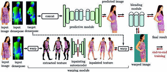
Overview of our pose transfer pipeline: given an input image and a target pose we use DensePose [1] to drive the generation process. This is achieved through the complementary streams of (a) a data-driven predictive module, and (b) a surface-based module that warps the texture to UV-coordinates, interpolates on the surface, and warps back to the target image. A blending module combines the complementary merits of these two streams in a single end-to-end trainable framework.
1 Introduction
Deep models have recently shown remarkable success in tasks such as face [2], human [3,4,5], or scene generation [6, 7], collectively known as “neural synthesis”. This opens countless possibilities in computer graphics applications, including cinematography, gaming and virtual reality settings. At the same time, the potential malevolent use of this technology raises new research problems, including the detection of forged images or videos [1. The war** module uses DensePose surface correspondence and inpainting to generate a new view of the person, while the predictive module is a generic, black-box, generative model conditioned on the DensePose outputs for the input and the target.
These modules corresponding to two parallel streams have complementary merits: the predictive module successfully exploits the dense conditioning output to generate plausible images for familiar poses, delivering superior results to those obtained from sparse, landmark-based conditioning; at the same time, it cannot generalize to new poses, or transfer texture details. By contrast, the war** module can preserve high-quality details and textures, allows us to perform inpainting in a uniform, canonical coordinate system, and generalizes for free for a broad variety of body movements. However, its body-, rather than clothing-centered construction does not take into account hair, hanging clothes, and accessories. The best of both worlds is obtained by feeding the outputs of these two blocks into a blending module trained to fuse and refine their predictions using a combination of reconstruction, adversarial, and perceptual losses in an end-to-end trainable framework.
The DensePose module is common to both streams and delivers dense correspondences between an image and a surface-based model of the human body. It does so by firstly assigning every pixel to one of 24 predetermined surface parts, and then regressing the part-specific surface coordinates of every pixel. The results of this system are encoded in three output channels, comprising the part label and part-specific UV surface coordinates. This system is trained discriminatively and provides a simple, feed-forward module for dense correspondence from an image to the human body surface. We omit further details, since we rely on the system of [1] with minor implementation differences described in Sect. 4.
Having outlined the overall architecture of our system, in Sects. 3.1 and 3.3 we present in some more detail our components, and then turn in Sect. 3.4 to the loss functions used in their training. A thorough description of architecture details is left to the supplemental material. We start by presenting the architecture of the predictive stream, and then turn to the surface-based stream, corresponding to the upper and lower rows of Fig. 1, respectively.
3.1 Predictive Stream
The predictive module is a conditional generative model that exploits the DensePose system results for pose transfer. Existing conditional models indicate the target pose in the form of heat-maps from keypoint detectors [4], or part segmentations [3]. Here we condition on the concatenation of the input image and DensePose results for the input and target images, resulting in an input of dimension \(256\, \times \, 256 \times 9\). This provides conditioning that is both global (part-classification), and point-level (continuous coordinates), allowing the remaining network to exploit a richer source of information.
The remaining architecture includes an encoder followed by a stack of residual blocks and a decoder at the end, along the lines of [28]. In more detail, this network comprises (a) a cascade of three convolutional layers that encode the \(256 \times 256 \times 9\) input into \(64 \times 64 \times 256\) activations, (b) a set of six residual blocks with \(3 \times 3 \times 256 \times 256 \) kernels, (c) a cascade of two deconvolutional and one convolutional layer that deliver an output of the same spatial resolution as the input. All intermediate convolutional layers have \(3{\times }3\) filters and are followed by instance normalization [36] and ReLU activation. The last layer has tanh non-linearity and no normalization.
3.2 War** Stream
Our war** module performs pose transfer by performing explicit texture map** between the input and the target image on the common surface UV-system. The core of this component is a Spatial Transformer Network (STN) [37] that warps according to DensePose the image observations to the UV-coordinate system of each surface part; we use a grid with \(256\ {\times }\ 256 \) UV points for each of the 24 surface parts, and perform scattered interpolation to handle the continuous values of the regressed UV coordinates. The inverse map** from UV to the output image space is performed by a second STN with a bilinear kernel. As shown in Fig. 3, a direct implementation of this module would often deliver poor results: the part of the surface that is visible on the source image is typically small, and can often be entirely non-overlap** with the part of the body that is visible on the target image. This is only exacerbated by DensePose failures or systematic errors around the part seams. These problems motivate the use of an inpainting network within the war** module, as detailed below.
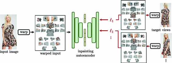
Supervision signals for pose transfer on the war** stream: the input image on the left is warped to intrinsic surface coordinates through a spatial transformer network driven by DensePose. From this input, the inpainting autoencoder has to predict the appearance of the same person from different viewpoints, when also warped to intrinsic coordinates. The loss functions on the right penalize the reconstruction only on the observed parts of the texture map. This form of multi-view supervision acts like a surrogate for the (unavailable) appearance of the person on the full body surface.
Inpainting Autoencoder. This model allows us to extrapolate the body appearance from the surface nodes populated by the STN to the remainder of the surface. Our setup requires a different approach to the one of other deep inpainting methods [33], because we never observe the full surface texture during training. We handle the partially-observed nature of our training signal by using a reconstruction loss that only penalizes the observed part of the UV map, and lets the network freely guess the remaining domain of the signal. In particular, we use a masked \(\ell _1\) loss on the difference between the autoencoder predictions and the target signals, where the masks indicate the visibility of the target signal.
We observed that by its own this does not urge the network to inpaint successfully; results substantially improve when we accompany every input with multiple supervision signals, as shown in Fig. 2, corresponding to UV-wrapped shots of the same person at different poses. This fills up a larger portion of the UV-space and forces the inpainting network to predict over the whole texture domain. As shown in Fig. 3, the inpainting process allows us to obtain a uniformly observed surface, which captures the appearance of skin and tight clothes, but does not account for hair, skirts, or apparel, since these are not accommodated by DensePose’s surface model.
Our inpainting network is comprised of N autoencoders, corresponding to the decomposition of the body surface into N parts used in the original DensePose system [1]. This is based on the observation that appearance properties are non-stationary over the body surface. Propagation of the context-based information from visible to invisible parts that are entirely occluded at the present view is achieved through a fusion mechanism that operates at the level of latent representations delivered by the individual encoders, and injects global pose context in the individual encoding through a concatenation operation.
In particular, we denote by \(\mathcal {E}_i\) the individual encoding delivered by the encoder for the i-th part. The fusion layer concatenates these obtained encodings into a single vector which is then down-projected to a 256-dimensional global pose embedding through a linear layer. We pass the resulting embedding through a cascade of ReLU and Instance-Norm units and transform it again into an embedding denoted by \(\mathcal {G}\).
Then the i-th part decoder receives as an input the concatenation of \(\mathcal {G}\) with \(\mathcal {E}_i\), which combines information particular to part i, and global context, delivered by \(\mathcal {G}\). This is processed by a stack of deconvolution operations, which delivers in the end the prediction for the texture of part i.
3.3 Blending Module
The blending module’s objective is to combine the complementary strengths of the two streams to deliver a single fused result, that will be ‘polished’ as measured by the losses used for training. As such it no longer involves an encoder or decoder unit, but rather only contains two convolutional and three residual blocks that aim at combining the predictions and refining their results.
In our framework, both predictive and war** modules are first pretrained separately and then finetuned jointly during blending. The final refined output is obtained by learning a residual term added to the output of the predictive stream. The blending module takes an input consisting of the outputs of the predictive and the war** modules combined with the target dense pose.
3.4 Loss Functions
As shown in Fig. 1, the training set for our network comes in the form of pairs of input and target images, \(\varvec{x}\), \(\varvec{y}\) respectively, both of which are of the same person-clothing, but in different poses. Denoting by \(\varvec{\hat{y}}=G(\varvec{x})\) the network’s prediction, the difference between \(\varvec{\hat{y}},\varvec{y}\) can be measured through a multitude of loss terms, that penalize different forms of deviation. We present them below for completeness and ablate their impact in practice in Sect. 4.
Reconstruction Loss. To penalize reconstruction errors we use the common \(\ell _1\) distance between the two signals: \(\Vert \varvec{\hat{y}} -\varvec{y}\Vert _1\). On its own, this delivers blurry results but is important for retaining the overall intensity levels.
Perceptual Loss. As in Chen and Koltun [6], we use a VGG19 network pretrained for classification [38] as a feature extractor for both \(\varvec{\hat{y}},\varvec{y}\) and penalize the \(\ell _2\) distance of the respective intermediate feature activations \(\varPhi ^{v}\) at 5 different network layers \(v=1,\ldots ,N\):
This loss penalizes differences in low- mid- and high-level feature statistics, captured by the respective network filters.
Style Loss. As in [28], we use the Gram matrix criterion of [25] as an objective for training a feedforward network. We first compute the Gram matrix of neuron activations delivered by the VGG network \(\varPhi \) at layer v for an image \(\varvec{x}\):
where h and w are horizontal and vertical pixel coordinates and c and \(c'\) are feature maps of layer v. The style loss is given by the sum of Frobenius norms for the difference between the per-layer Gram matrices \(\mathcal {G}^{v}\) of the two inputs:
Adversarial Loss. We use adversarial training to penalize any detectable differences between the generated and real samples. Since global structural properties are largely settled thanks to DensePose conditioning, we opt for the patchGAN [12] discriminator, which operates locally and picks up differences between texture patterns. The discriminator [7, 12] takes as an input \(\varvec{z}\), a combination of the source image and the DensePose results on the target image, and either the target image \(\varvec{y}\) (real) or the generated output (fake) \(\varvec{\hat{y}}\). We want fake samples to be indistinguishable from real ones – as such we optimize the following objective:
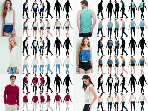
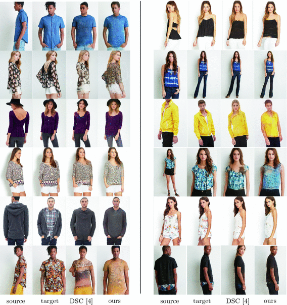
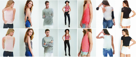
where we use \(l(x) = x^2\) as in the Least Squares GAN (LSGAN) work of [4.1 Implementation Details DensePose Estimator. We use a fully convolutional network (FCN) similar to the one used as a teacher network in [1]. The FCN is a ResNet-101 trained on cropped person instances from the COCO-DensePose dataset. The output consists of 2D fields representing body segments (I) and \(\{U,V\}\) coordinates in coordinate spaces aligned with each of the semantic parts of the 3D model. Training Parameters. We train the network and its submodules with Adam optimizer with initial learning rate \(2\,{\cdot }\,10^{-4}\) and \(\beta _1\,{=}\,0.5\), \(\beta _2\,{=}\,0.999\) (no weight decay). For speed, we pretrain the predictive module and the inpainting module separately and then train the blending network while finetuning the whole combined architecture end-to-end; DensePose network parameters remain fixed. In all experiments, the batch size is set to 8 and training proceeds for 40 epochs. The balancing weights \(\lambda \) between different losses in the blending step (described in Sect. 3.4) are set empirically to \(\lambda _{\ell _1}=1\), \(\lambda _{\text {p}}=0.5\), \(\lambda _{\text {style}}=5\,{\cdot }\,10^{5}\), \(\lambda _{\text {GAN}}=0.1\). As of today, there exists no general criterion allowing for adequate evaluation of the generated image quality from the perspective of both structural fidelity and photorealism. We therefore adopt a number of separate structural and perceptual metrics widely used in the community and report our joint performance on them. Structure. The geometry of the generations is evaluated using the perception-correlated Structural Similarity metric (SSIM) [40]. We also exploit its multi-scale variant MS-SSIM [43] to estimate the geometry of our predictions at a number of levels, from body structure to fine clothing textures. Image Realism. Following previous works, we provide the values of Inception scores (IS) [41]. However, as repeatedly noted in the literature, this metric is of limited relevance to the problem of within-class object generation, and we do not wish to draw strong conclusions from it. We have empirically observed its instability and high variance with respect to the perceived quality of generations and structural similarity. We also note that the ground truth images from the DeepFashion dataset have an average IS of 3.9, which indicates low degree of realism of this data according to the IS metric (for comparison, IS of CIFAR-10 is 11.2 [41] with best image generation methods achieving IS of 8.8 [2]). In addition, we perform additional evaluation using detection scores (DS) [5] reflecting the similarity of the generations to the person class. Detection scores correspond to the maximum of confidence of the PASCAL-trained SSD detector [44] in the person class taken over all detected bounding boxes. Qualitative comparison with the state-of-the-art Deformable GAN (DSC) method of [5]. Each group shows the input, the target image, DSC predictions [5], predictions obtained with our full model. We observe that even though our cloth texture is occasionally not as sharp, we better retain face, gender, and skin color information. We first compare the performance of our framework to a number of recent methods proposed for the task of keypoint guided image generation or multi-view synthesis. Table 1 shows a significant advantage of our pipeline in terms of structural fidelity of obtained predictions. This holds for the whole range of tested network configurations and training setups (see Table 4). In terms of perceptional quality expressed through IS, the output generations of our models are of higher quality or directly comparable with the existing works. Some qualitative results of our method (corresponding to the balanced model in Table 1) and the best performing state-of-the-art approach [5] are shown in Fig. 4. We have also performed a user study on Amazon Mechanical Turk, following the protocol of [5]: we show 55 real and 55 generated images in a random order to 30 users for one second. As the experiment of [5] was done with the help of fellow researchers and not AMT users, we perform an additional evaluation of images generated by [5] for consistency, using the official public implementation. We perform three evaluations, shown in Table 1: Realism asks users if the image is real or fake. Anatomy asks if a real, or generated image is anatomically plausible. Pose shows a pair of a target and a generated image and asks if they are in the same pose. The results (correctness, in %) indicate that generations of [5] have higher degree of perceived realism, but our generations show improved pose fidelity and higher probability of overall anatomical plausibility. In order to clearly measure the effectiveness of the DensePose-based conditioning, we first compare to the performance of the ‘black box’, predictive module when used in combination with more traditional body representations, such as background/foreground masks, body part segmentation maps or body landmarks. As a segmentation map we take the index component of DensePose and use it to form a one-hot encoding of each pixel into a set of class specific binary masks. Accordingly, as a background/foreground mask, we simply take all pixels with positive DensePose segmentation indices. Finally, following [5] we use [39] to obtain body keypoints and one-hot encode them. In each case, we train the predictive module by concatenating the source image with a corresponding representation of the source and the target poses which results in 4 input planes for the mask, 27 for segmentation maps and 21 for the keypoints. The corresponding results shown in Table 2 demonstrate a clear advantage of fine-grained dense conditioning over the sparse, keypoint-based, or coarse, segmentation-based, representations. Complementing these quantitative results, typical failure cases of keypoint-based frameworks are demonstrated in Fig. 5. We observe that these shortcomings are largely fixed by switching to the DensePose-based conditioning. Table 3 shows the contribution of each of the predictive module, war** module, and inpainting autoencoding blocks in the final model performance. For these experiments, we use only the reconstruction loss \(\mathcal {L}_{\ell _1}\), factoring out fluctuations in the performance due to instabilities of GAN training. As expected, including the war** branch in the generation pipeline results in better performance, which is further improved by including the inpainting in the UV space. Qualitatively, exploiting the inpainted representation has two advantages over the direct war** of the partially observed texture from the source pose to the target pose: first, it serves as an additional prior for the fusion pipeline, and, second, it also prevents the blending network from generating clearly visible sharp artifacts that otherwise appear on the boarders of partially observed segments of textures. In Table 4 we analyze the role of each of the considered terms in the composite loss function used at the final stage of the training, while providing indicative results in Fig. 6. The perceptual loss \(\mathcal {L}_p\) is most correlated with the image structure and least correlated with the perceived realism, probably due to introduced textural artifacts. At the same time, the style loss \(\mathcal {L}_{\text {style}}\) produces sharp and correctly textured patterns while hallucinating edges over uniform regions. Finally, adversarial training with the loss \(\mathcal {L}_{\text {GAN}}\) tends to prioritize visual plausibility but often disregarding structural information in the input. This justifies the use of all these complimentary supervision criteria in conjunction, as indicated in the last entry of Table 4.4.2 Evaluation Metrics
4.3 Comparison with the State-of-the-Art
4.4 Effectiveness of Different Body Representations
4.5 Ablation Study on Architectural Choices
4.6 Ablation Study on Supervision Objectives
5 Conclusion
In this work we have introduced a two-stream architecture for pose transfer that exploits the power of dense human pose estimation. We have shown that dense pose estimation is a clearly superior conditioning signal for data-driven human pose estimation, and also facilitates the formulation of the pose transfer problem in its natural, body-surface parameterization through inpainting. In future work we intend to further pursue the potential of this method for photorealistic image synthesis [2, 6] as well as the treatment of more categories.
References
Guler, R.A., Neverova, N., Kokkinos, I.: Densepose: dense human pose estimation in the wild. In: CVPR (2018)
Karras, T., Aila, T., Samuli, L., Lehtinen, J.: Progressive growing of gans for improved quality, stability, and variation. In: ICLR (2018)
Lassner, C., Pons-Moll, G., Gehler, P.V.: A generative model of people in clothing. In: ICCV (2017)
Ma, L., Jia, X., Sun, Q., Schiele, B., Tuytelaars, T., Van Gool, L.: Pose guided person image generation. In: NIPS (2017)
Siarohin, A., Sangineto, E., Lathuiliere, S., Sebe, N.: Deformable gans for pose-based human image generation. In: CVPR (2018)
Chen, Q., Koltun, V.: Photographic image synthesis with cascaded refinement networks. In: ICCV (2017)
Wang, T.C., Liu, M.Y., Zhu, J.Y., Tao, A., Jan, K., Bryan, C.: High-resolution image synthesis and semantic manipulation with conditional gans. In: CVPR (2018)
Rossler, A., Cozzolino, D., Verdoliva, L., Riess, C., Thies, J., Niener, M.: Faceforensics: a large-scale video dataset for forgery detection in human faces. ar**v:1803.09179v1 (2018)
Shrivastava, A., Pfister, T., Tuzel, O., Susskind, J., Weng, W., Webb, R.: Learning from simulated and unsupervised images through adversarial training. In: CVPR (2017)
Lample, G., Zeghidour, N., Usunier, N., Bordes, A., Denoyer, L., Ranzato, M.: Fader networks: manipulating images by sliding attributes. In: NIPS (2017)
Shu, Z., Yumer, E., Hadap, S., Sunkavalli, K., Shechtman, E., Samaras, D.: Neural face editing with intrinsic image disentangling. In: CVPR (2017)
Isola, P., Zhu, J., Zhou, T., Efros, A.A.: Image-to-image translation with conditional adversarial networks. In: CVPR (2017)
Loper, M., Mahmood, N., Romero, J., Pons-Moll, G., Black, M.J.: SMPL: a skinned multi-person linear model. ACM Trans. Graph. 34(6), 248:1–248:16 (2015). (Proc. SIGGRAPH Asia)
Bogo, F., Kanazawa, A., Lassner, C., Gehler, P., Romero, J., Black, M.J.: Keep It SMPL: automatic estimation of 3D human pose and shape from a single image. In: Leibe, B., Matas, J., Sebe, N., Welling, M. (eds.) ECCV 2016. LNCS, vol. 9909, pp. 561–578. Springer, Cham (2016). https://doi.org/10.1007/978-3-319-46454-1_34
Lassner, C., Romero, J., Kiefel, M., Bogo, F., Black, M.J., Gehler, P.V.: Unite the people: closing the loop between 3D and 2D human representations. In: ICCV (2017)
Varol, G., et al.: Learning from synthetic humans. In: CVPR (2017)
Kanazawa, A., Black, M.J., Jacobs, D.W., Malik, J.: End-to-end recovery of human shape and pose. In: CVPR (2018)
Guler, R.A., Trigeorgis, G., Antonakos, E., Snape, P., Zafeiriou, S., Kokkinos, I.: Densereg: fully convolutional dense shape regression in-the-wild. In: CVPR (2017)
Liu, Z., Luo, P., Qiu, S., Wang, X., Tang, X.: Deepfashion: powering robust clothes recognition and retrieval with rich annotations. In: CVPR (2016)
Liu, K.H., Chen, T.Y., Chen, C.S.: A dataset for view-invariant clothing retrieval and attribute prediction. In: ICMR (2016)
Hinton, G.E., Salakhutdinov, R.R.: Reducing the dimensionality of data with neural networks. Science 313(5786), 504–507 (2006)
Kingma, D.P., Welling, M.: Auto-encoding variational bayes. In: ICLR (2014)
Goodfellow, I., et al.: Generative adversarial nets. In: NIPS (2014)
Radford, A., Metz, L., Chintala, S.: Unsupervised representation learning with deep convolutional generative adversarial networks. In: ICLR (2016)
Gatys, L.A., Ecker, A.S., Bethge, M.: A neural algorithm of artistic style. In: CVPR (2016)
Mao, X., Li, Q., **e, H., Lau, R.Y., Wang, Z., Smolley, S.P.: Least squares generative adversarial networks. In: ICCV (2017)
Arjovsky, M., Chintala, S., Bottou, L.: Wasserstein generative adversarial networks. In: ICML (2017)
Johnson, J., Alahi, A., Fei-Fei, L.: Perceptual losses for real-time style transfer and super-resolution. In: Leibe, B., Matas, J., Sebe, N., Welling, M. (eds.) ECCV 2016. LNCS, vol. 9906, pp. 694–711. Springer, Cham (2016). https://doi.org/10.1007/978-3-319-46475-6_43
Ulyanov, D., Lebedev, V., Vedaldi, A., Lempitsky, V.: Texture networks: feed-forward synthesis of textures and stylized images. In: ICML (2016)
Zhu, S., Fidler, S., Urtasun, R., Lin, D., Loy, C.C.: Be your own prada: fashion synthesis with structural coherence. In: ICCV (2017)
Zhao, B., Wu, X., Cheng, Z.Q., Liu, H., Feng, J.: Multi-view image generation from a single-view. In: ACM on Multimedia Conference (2018)
Pathak, D., Krähenbühl, P., Donahue, J., Darrell, T., Efros, A.A.: Context encoders: feature learning by inpainting. In: CVPR (2016)
Yeh, R.A., Chen, C., Lim, T., Hasegawa-Johnson, M., Do, M.N.: Semantic image inpainting with perceptual and contextual losses. In: CVPR (2017)
Saito, S., Wei, L., Hu, L., Nagano, K., Li, H.: Photorealistic facial texture inference using deep neural networks. In: CVPR (2017)
Deng, J., Cheng, S., Xue, N., Zhou, Y., Zafeiriou, S.: UV-GAN: adversarial facial UV map completion for pose-invariant face recognition. In: CVPR (2018)
Ulyanov, D., Vedaldi, A., Lempitsky, V.: Improved texture networks: maximizing quality and diversity in feed-forward stylization and texture synthesis. In: CVPR (2017)
Jaderberg, M., Simonyan, K., Zisserman, A., Kavukcuoglu, K.: Spatial transformer networks. In: NIPS (2015)
Simonyan, K., Zisserman, A.: Very deep convolutional networks for large-scale image recognition. In: ICLR (2015)
Cao, Z., Simon, T., Wei, S., Sheikh, Y.: Realtime multiperson 2D pose estimation using part affinity fields. In: CVPR (2017)
Wang, Z., Bovik, A.C., Sheikh, H.R., Simoncelli, E.P.: Image quality assessment: from error visibility to structural similarity. In: TIP (2004)
Salimans, T., Goodfellow, I., Zaremba, W., Cheung, V., Radford, A., Chen, X.: Improved techniques for training gans. In: NIPS (2016)
Ma, L., Sun, Q., Georgoulis, S., Van Gool, L., Schiele, B., Fritz, M.: Disentangled person image generation. In: CVPR (2018)
Wang, Z., Simoncelli, E.P., Bovik, A.C.: Multi-scale structural similarity for image quality assessment. In: ACSSC (2003)
Liu, W., et al.: SSD: Single shot multibox detector. In: Leibe, B., Matas, J., Sebe, N., Welling, M. (eds.) ECCV 2016. LNCS, vol. 9905, pp. 21–37. Springer, Cham (2016). https://doi.org/10.1007/978-3-319-46448-0_2
Author information
Authors and Affiliations
Corresponding author
Editor information
Editors and Affiliations
1 Electronic supplementary material
Below is the link to the electronic supplementary material.
Rights and permissions
Copyright information
© 2018 Springer Nature Switzerland AG
About this paper
Cite this paper
Neverova, N., Alp Güler, R., Kokkinos, I. (2018). Dense Pose Transfer. In: Ferrari, V., Hebert, M., Sminchisescu, C., Weiss, Y. (eds) Computer Vision – ECCV 2018. ECCV 2018. Lecture Notes in Computer Science(), vol 11207. Springer, Cham. https://doi.org/10.1007/978-3-030-01219-9_8
Download citation
DOI: https://doi.org/10.1007/978-3-030-01219-9_8
Published:
Publisher Name: Springer, Cham
Print ISBN: 978-3-030-01218-2
Online ISBN: 978-3-030-01219-9
eBook Packages: Computer ScienceComputer Science (R0)


