
Abstract
We present a framework for efficient stateless model checking (SMC) of concurrent programs under three prominent models of causal consistency, \({\texttt {CCv}}, {\texttt {CM}}, \texttt{CC}\). Our approach is based on exploring traces under the program order  and the reads from
  relations. Our SMC algorithm is provably optimal in the sense that it explores each
  and
and  relation exactly once. We have implemented our framework in a tool called Conschecker. Experiments show that Conschecker performs well in detecting anomalies in classical distributed databases benchmarks.
You have full access to this open access chapter, Download conference paper PDF
1 Introduction
Traditionally, distributed shared memories ensure that all processes in the system agree on a common order of all operations on memory. Such guarantees are provided by sequential consistency (SC) [33], and by linearizable memory [26]. However, providing these consistency guarantees entails access latencies, making them inefficient for large systems. There is a tradeoff in providing strong consistency guarantees while ensuring low latency and this presents significant efficiency challenges. There is a large body of work which suggests that a systematic weakening of memory consistency can reduce the costs of providing consistency. Weakened consistency guarantees admit more concurrent behaviours than SC or linearizability. To this end, Lamport [32] proposed causal consistency which provides an ordering among events in a distributed system in which processes communicate via message passing. This has been adapted [7] to a setting of reads and writes in a shared memory environment. In this setting, the return values of reads must be consistent with causally related reads and writes. As causality only orders events partially, the reading processes can disagree on the relative ordering of concurrent writes. This makes concurrent writer processes independent, reducing the costs of synchronization.
Several efforts have been made to formalize causal consistency [16, 25, 39] [7, 8, 10, 15, 38, 40] and there are many implementations [9, 20, 21] satisfying this criterion as opposed to strong consistency (linearizability).
While strong consistency makes it easier to program than weak ones, they require costly implementations. Weak memories may be easier to implement, but much harder to program. An acceptable medium which has emerged over the years are three important notions in causal consistency, respectively causal consistency (\(\texttt{CC}\)) [15, 25], causal convergence (\(\texttt {CCv}\)) [15, 16, 25, 39] and causal memory (\({\texttt {CM}}\)) [7, 15, 25, 39].
The focus of this paper is the verification of shared memory programs under causal consistency. We consider the three variants mentioned above. We propose a stateless model checking (SMC) framework that covers all three variants. SMC is a successful technique for finding concurrency bugs [23]. For a terminating program, SMC systematically explores all process schedulings that are possible during runs of the program. The number of possible schedulings grows exponentially with the execution length in SMC. To counter this and reduce the number of explored executions, the technique of partial order reduction [18, 22] has been proposed. This has been adapted to SMC as DPOR (dynamic partial order reduction). DPOR was first developed for concurrent programs under SC [1, 41]. Recent years have seen DPOR adapted to language induced weak memory models [28, 37, 5], as well as hardware-induced relaxed memory models [3, 46]. To the best of our knowledge, DPOR algorithms have not been developed for causal consistency models. The goal of this paper is to fill this gap.
DPOR is based on the observation that two executions are equivalent if they induce the same ordering between conflicting events, and hence it is sufficient to consider one such execution from each equivalence class. Under sequential consistency, these equivalence classes are called Mazurkiewicz traces [34], while for relaxed memory models, the generalization of these are called Shasha-Snir traces [42]. A Shasha-Snir trace characterizes an execution of a concurrent program by the relations (1)  program order, which totally orders events of each process, (2),
  reads from, which connects each read with the write it reads from, (3)
  coherence order, which totally orders writes to the same shared variable. DPOR can be optimized further by observing that the assertions to be verified at the end of an execution does not depend on the coherence order of shared variables, and hence it suffices to consider traces over
  . Based on this observation, the DPOR algorithms for programs under the release-acquire semantics (RA) and SC [4, 5] explores traces with
  and
and  where the
  edges are added on the fly. The equivalence classes are considered wrt
  , reducing the number of distinct traces to be analyzed.
Contributions. We propose a DPOR based SMC algorithm for all three consistency models \(\texttt{CC}, {\texttt {CCv}}, {\texttt {CM}}\) which explores systematically, all the distinct  traces covering all possible executions of the program. We develop a uniform algorithm for all three models which is sound and complete : that is, all traces explored are consistent wrt the model \(X \in \{\texttt{CC}, {\texttt {CCv}}, {\texttt {CM}}\}\) under consideration, and all such consistent traces are explored. Moreover, our algorithm is optimal in the sense that, each consistent
  trace is explored exactly once. One of the key challenges during the trace exploration is to maintain the consistency of the traces wrt the model under consideration. We tackle this by defining a trace semantics which ensures that the traces generated in each step only contain edges which will be present in any consistent trace. We implement our algorithms in a tool Conschecker which is, to the best of our knowledge, the first of its kind to perform SMC on the three prominent causal consistency models \(\texttt{CC}, {\texttt {CCv}}, {\texttt {CM}}\). Conschecker checks for assertion violation of programs under \(\texttt{CC}, {\texttt {CCv}}, {\texttt {CM}}\). We evaluate the correctness of our tool on \(\texttt{CC}, {\texttt {CCv}}, {\texttt {CM}}\) by simulating these models on the memory model simulator Herd [8] and validating our outcomes with theirs. Then we proceed with experimental evaluation on a wide range of benchmarks from distributed databases. We showed that (i) \(\textsc {Conschecker}\) correctly detects known consistency bugs [12,13,14] and [11] under \({\texttt {CCv}}, {\texttt {CM}}, \texttt{CC}\), (ii) \(\textsc {Conschecker}\) correctly detects known assertion violations in applications [12, 19, 27, 36]. We also did a stress test of Conschecker on some SV-COMP benchmarks and parameterized benchmarks which resulted in a large number (6 million) of traces.
Related Work. SMC has been implemented in many tools CHESS [35], Concuerror [17], VeriSoft [24], Nidhugg [3], CDSChecker [37], RCMC[28], GenMC [30], rInspect [46] and Tracer [5]. While most of these work with either Mazurkewicz traces or  traces, [6] proposes a RVF-SMC algorithm where the value read is used to decide equivalence of two runs.
In recent years, there has been much interest in DPOR algorithms : [4] for SC, [30] for the release acquire semantics, [43] for C/C++, and [29] for TSO, PSO and RC11. It is known that \(\texttt{CC}\) is weaker than RA, \({\texttt {CCv}}\) is stronger than RA while \({\texttt {CM}}\) is incomparable with RA [31]. In conclusion, all the above memory models are different from \(\texttt{CC}, {\texttt {CCv}}, {\texttt {CM}}\). Hence we cannot reuse any of the existing DPOR algorithms.
Recent work on causal consistency [15] studies the complexity of checking whether one execution (all executions) of a program under \(\texttt{CC}, {\texttt {CCv}}, {\texttt {CM}}\) is consistent. They show that checking if an execution is consistent is NP-completeness, while the question of checking if all executions are consistent is undecidable. [11, 12] explore the robustness wrt SC, of transactional programs under \(\texttt{CC}, {\texttt {CCv}}, {\texttt {CM}}\). However, none of these papers propose a DPOR algorithm for \(\texttt{CC}, {\texttt {CCv}}, {\texttt {CM}}\).
2 Preliminaries
 We consider a program \({\mathcal P}\) consisting of a finite set \({\mathcal T}\) of threads (processes) that share a finite set \({\mathbb {X}}\) of (shared) variables, ranging over a domain \({\mathbb V}\) of values that includes a special value \(0\).
A process has a finite set of local registers that store values from \({\mathbb V}\). Each process runs a deterministic code, built in a standard way from expressions and atomic commands, using standard control flow constructs (sequential composition, selection, and bounded loop constructs). Throughout the paper, we use \(x, y\) for shared variables, \({\texttt {a}}, {\texttt {b}}, {\texttt {c}}\) for registers, and \(e\) for expressions. Global statements are either writes \(x:=e\) to a shared variable, or reads \({\texttt {a}}:=x\) from a shared variable. Local statements only access and affect the local state of the process and include assignments \({\texttt {a}}:=e\) to registers, and conditional control flow constructs. Note that expressions do not contain shared variables, implying that a statement accesses at most one shared variable.
The local state of a process \({ proc}\in {\mathcal T}\) is defined by its program counter and the contents of its registers. A configuration of \({\mathcal P}\) is made up of the local states of all the processes. The values of the shared variables are not part of a configuration. A program execution is a sequence of transitions between configurations, starting with the initial configuration \(\gamma ^{\textsf{init}}\). Each transition corresponds to one process performing a local or global statement. A transition between two configurations \(\gamma \) and \(\gamma '\) is of form \(\gamma {\mathop {\leadsto }\limits ^{\ell }}\gamma '\), where the label \(\ell \) describes the interaction with shared variables. The label \(\ell \) is one of three forms: (i) \(\left\langle { proc},\varepsilon \right\rangle \), indicating a local statement performed by thread \({ proc}\), which updates only the local state of \({ proc}\), (ii) \(\left\langle { proc},{\textsf{wt}},x,v\right\rangle \), indicating a write of the value \(v\) to the variable \(x\) by the thread \({ proc}\), which also updates the program counter of \({ proc}\), and (iii) \(\left\langle { proc},{\textsf{rd}},x,v\right\rangle \) indicating a read of \(v\) from \(x\) by the thread \({ proc}\) into some register, while also updating the program counter of \({ proc}\). There is no constraint on the values that are used in transitions corresponding to read statements. This will allow some illegal program behaviors, which is sorted by associating runs with so-called traces, which represent how reads obtain their values from writes. A causal consistency model \(X \in \{\texttt{CC}, {\texttt {CCv}}, {\texttt {CM}}\}\) is formulated by imposing restrictions on traces, thereby also restricting the possible runs that are associated with them.
Since local statements are not visible to other threads, we will not represent them explicitly in the transition relation considered in our DPOR algorithm. Instead, we let each transition represent the combined effect of some finite sequence of local statements by a process followed by a global statement by the same process. For configurations \(\gamma \) and \(\gamma '\) and a label \(\ell \) which is either of the form \(\left\langle { proc},{\textsf{wt}},x,v\right\rangle \) or of the form \(\left\langle { proc},{\textsf{rd}},x,v\right\rangle \), we let \(\gamma \xrightarrow {\ell }{}\gamma '\) denote that we can reach \(\gamma '\) from \(\gamma \) by performing a sequence of transitions labeled with \(\left\langle { proc},\varepsilon \right\rangle \) followed by a transition labeled with \(\ell \). Defining the relation \(\xrightarrow {}{}\) in this manner ensures that we take the effect of local statements into account, while avoiding consideration of interleavings of local statements of different threads in the analysis.
We use \(\gamma \xrightarrow {}{}\gamma '\) to denote that \(\gamma \xrightarrow {\ell }{}\gamma '\) for some \(\ell \) and define \(\texttt{succ}\!\left( \gamma \right) := \left\{ {\gamma '}\mid {\gamma \xrightarrow {}{}\gamma '}\right\} \), i.e., it is the set of successors of \(\gamma \) wrt. \(\xrightarrow {}{}\). A configuration \(\gamma \) is said to be terminal if \(\texttt{succ}\!\left( \gamma \right) =\emptyset \), i.e., no thread can execute a global statement from \(\gamma \). A run \(\rho \) from \(\gamma \) is a sequence \(\gamma _0\xrightarrow {\ell _1}{}\gamma _1 \xrightarrow {\ell _2}{}\cdots \xrightarrow {\ell _n}{} \gamma _n\) such that \(\gamma _0=\gamma \). We say that \(\rho \) is terminated if \(\gamma _n\) is terminal. We let \({ Runs}(\gamma )\) denote the set of runs from \(\gamma \).
 . An event corresponds to a particular execution of a statement in a run of \({\mathcal P}\). A write event \( ev \) is given by \((id,{ proc},\textsf{wt}(x,v))\) where \(id \in {\mathbb N}\) is the identifier of the event, \({ proc}\) is the process containing the event, \(x\in {\mathbb {X}}\) is a variable, and \(v\in {\mathbb V}\) is a value. This event corresponds to a process writing the value \(v\) to variable \(x\). Likewise, a read event \( ev \) is given by \((id, { proc}, \textsf{rd}(x))\) where \(x\in {\mathbb {X}}\). This event corresponds to a process reading some value to \(x\). The read event \( ev \) does not specify the particular value it reads; this value will be defined in a trace by specifying a write event from which \( ev \) fetches its value. For each variable \(x\in {\mathbb {X}}\), we assume a special write event \(\textsf{init}_{x}=\textsf{wt}(x,0)\) called the initializer event for \(x\). This event is not performed by any of the processes in \({\mathcal T}\), and writes the value \(0\) to \(x\). We define \(\texttt{E}_{{ init}}:=\left\{ {\textsf{init}_{x}}\mid {x\in {\mathbb {X}}}\right\} \) as the set of initializer events. If \(\texttt{E}\) is a set of events, we define subsets of \(\texttt{E}\) characterized by particular attributes of its events. For instance, for a variable \(x\), we let \(\texttt{E}^{{\textsf{wt}},x}\) denote \(\left\{ { ev \in \texttt{E}}\mid {{ ev }.{ type}={\textsf{wt}}\wedge { ev }.{ var}=x}\right\} \).
 . A trace \(\tau \) is a tuple
  , where \(\texttt{E}\) is a set of events which includes the set \(\texttt{E}_{{ init}}\) of initializer events, and
  (program order),
  (read-from) are binary relations on \(\texttt{E}\) that satisfy:
-
 if \( process ( ev ) = process ( ev ')\) and \( ev .id < ev '.id\).
  totally orders the events of each individual process.
 -
 if \( ev \) is a write event and \( ev '\) is a read event on the same variable, which obtains its value from \( ev \).
 if
if  totally orders the events of each individual process.
 if
if We can view  as a graph whose nodes are \(\texttt{E}\) and whose edges are defined by the relations
  ,
,  .
.  depicted by red solid edges captures the order in each process while
  edges are depicted as solid blue edges. We define the empty trace \(\tau _\emptyset :=\left\langle \texttt{E}_{{ init}},\emptyset ,\emptyset \right\rangle \), i.e., it contains only the initializer events, and all the relations are empty.
We define when a trace can be associated with a run. Consider a run \(\rho \) of form \(\gamma _0\xrightarrow {\ell _1}{}\cdots \xrightarrow {\ell _n}{}\gamma _n\), where \(\ell _i=\left\langle { proc}_i,\mathfrak {t}_i,x_i,v_i\right\rangle \), and let  be a trace. We write \(\rho \models \tau \) to denote that the following conditions are satisfied: (i) \(\texttt{E}=\{{ ev _1,\ldots , ev _n}\}\), i.e., each event corresponds exactly to one label in \(\rho \). (ii) If \(\ell _i=\left\langle { proc}_i,{\textsf{wt}},x_i,v_i\right\rangle \), then \( ev _i=\left\langle { id}_i,{ proc}_i,{\textsf{wt}},x_i,v_i\right\rangle \), and if \(\ell _i=\left\langle { proc}_i,{\textsf{rd}},x_i,v_i\right\rangle \), then \( ev _i=\left\langle { id}_i,{ proc}_i,{\textsf{rd}},x_i\right\rangle \). An event and its label do the same (write or read) on identical variables, and for writes, they also agree on the written value. (iii) \({ id}_i=| \left\{ {j}\mid {(1\le j\le i)\wedge ({ proc}_j={ proc}_i)}\right\} |\). \( ev .id\) shows how it is ordered relative to the other events of \( process ( ev )\). (iv) if
  then \(x_i=x_j\) and \(v_i=v_j\). (v) if
  then \(v_i=0\), i.e., \( ev _i\) reads the initial value of \(x\) which is \(0\).
3 Causally Consistent Models
We study three variants [15] of causal consistency : \(\texttt{CC}, {\texttt {CCv}}\) and \({\texttt {CM}}\). To define the three models formally, we introduce a function that, for each model, extends a given trace uniquely by a set of new edges. Then we define the model by requiring that the extended trace does not contain any cycles. A run of the program satisfies a consistency model X if its associated extended trace has no cycles.
Let \(\textsf{CO}\), called causality order represent  . Two events \(e_1, e_2\) are causally related if either \(e_1~\textsf{CO}~e_2\) or \(e_2~\textsf{CO}~e_1\).

Programs showing the differences between consistency models. The  denotes the expected return value of the read event.

solid red, blue edges are  , \(\textsf{wt}(x,v)\) and \(\textsf{rd}(x)\) are write, read events.
Causal Consistency \(\texttt{CC}\). We start presenting the weakest notion of causal consistency, \(\texttt{CC}\) [7, 25]. First we give an intuitive description of \(\texttt{CC}\). In \(\texttt{CC}\), events which are not causally related can be executed in different orders in different processes; moreover decisions made about these orders can be revised by each process. To illustrate, consider the program Fig.1(b). The write events \(\textsf{wt}(x,1), \textsf{wt}(x,2)\) are not causally related and hence can be ordered in any way. Note that \(p_b\) first orders \(x:=1\) after \(x:=2\) and reads 1 into \(\mathtt{{a}}\); it then revises this order, and orders \(x:=2\) after \(x:=1\) and reads 2 into \(\mathtt{{b}}\).
A trace \(\tau \) does not violate \(\texttt{CC}\) as long as there is a causality order which explains the return value of each read event.
To capture traces violating \(\texttt{CC}\), we define a relation  (for overwrite) on writes to the same variable. For any two writes \(w_1, w_2\) and a read r on a same variable, if \(w_1~\textsf{CO}~w_2~\textsf{CO}~r\), and
  , then
  . This says that r reads the overwritten write \(w_1\), resulting in a
  cycle. We refer to
  cycles as \(\textsf{CCcycle}\). We define a function \(\textsf{extend}_{\texttt{CC}}(\tau )\) which extends a trace
  by adding all possible
  edges between write events on the same variable. For a trace
  , we say that \(\tau \models \texttt{CC}\) iff \(\textsf{extend}_{\texttt{CC}}(\tau )\) does not have a \(\textsf{CCcycle}\).
 . Program Fig. 1(a) is not \(\texttt{CC}\) since there is no causality order which explains the return values of the read events. If we consider any trace (Fig. 2) of the program Fig.1(a), we find that
  where \(r=\textsf{rd}(y)\),
  ,
,  . Then we get \(\textsf{wt}(x,1) ~\textsf{CO}~ \textsf{wt}(x,2)\), \(\textsf{wt}(x,2) ~\textsf{CO}~r'\) where \(r'=\textsf{rd}(x)\) and
  giving
  witnessing \(\textsf{CCcycle}\).
Causal Convergence \({\texttt {CCv}}\). Under \({\texttt {CCv}}\), we need a total order on all write events per variable. This order, called arbitration order, is an abstraction of how conflicts are resolved by all processes to agree upon one ordering among events which are not causally related. Thus, unlike \(\texttt{CC}\), a process cannot revise its ordering of the events which are not causally related, and all processes must follow one ordering. This makes it stronger than \(\texttt{CC}\).
To enforce a total order between all writes, we use a new relation  called conflict relation on all write events per variable. For all variables \(x \in \mathcal {V}\), and writes \(w_1,w_2\) on x and a read \(r=\textsf{rd}(x)\), if \(w_1 ~\textsf{CO}~r\), and
  then
then  . We define a function \(\textsf{extend}_{{\texttt {CCv}}}(\tau )\) which extends a trace
  by adding all possible
  edges between write events on the same variable. Traces violating \({\texttt {CCv}}\) exhibit a
  cycle in \(\textsf{extend}_{{\texttt {CCv}}}(\tau )\), which we refer to as \(\textsf{CCvcycle}\). We say that \(\tau \models {\texttt {CCv}}\) iff \( \textsf{extend}_{{\texttt {CCv}}}(\tau )\) does not contain a \(\textsf{CCvcycle}\).
 . For the program Fig.1(b) and any trace \(\tau \), \(\textsf{extend}_{{\texttt {CCv}}}(\tau )\) has a \(\textsf{CCvcycle}\) (see Fig.2) since in any trace, we have \(w_1=\textsf{wt}(x,1)~\textsf{CO}~r_2\) where \(r_2=\textsf{rd}(x)\) and
  for \(w_2=\textsf{wt}(x,2)\) giving
  . We also have \(\textsf{wt}(x,2)~\textsf{CO}~r_1\) where \(r_1=\textsf{rd}(x)\) with
  giving
  . Intuitively, we cannot find a total order amongst the writes to justify the reads of 1 and 2.
However, the program Fig.1(c) has a trace \(\tau \) s.t. \(\textsf{extend}_{{\texttt {CCv}}}(\tau )\) does not have \(\textsf{CCvcycle}\). In the corresponding run, we first allow \(p_a\) to complete execution, followed by \(p_b\).
Causal Memory \({\texttt {CM}}\). The \({\texttt {CM}}\) model is stronger than \(\texttt{CC}\) and incomparable to \({\texttt {CCv}}\). Like \(\texttt{CC}\), in \({\texttt {CM}}\) also, a process can diverge from another one in its ordering of events which are not causally related. However, once a process chooses an ordering of such events, it cannot revise it; this makes it stronger than \(\texttt{CC}\) and incomparable to \({\texttt {CCv}}\).
A happened before relation per process fixes the per process ordering of events. For a read/write event e in a trace, the Causal Past of e, \(\textsf{Causal Past}(e)=\{e' \mid e' ~\textsf{CO}~e\}\) is the set of events which are in the causal past of e. For an event e, the happened before relation  [15] is the smallest relation on events which is transitive, and is such that for all events \(e_1, e_2 \in \) \(\textsf{Causal Past}(e)\),
  . In other words,
  :
:  contains all pairs of events obtained by restricting \(\textsf{CO}\) to the events in the causal past of e. For any variable x, if we have writes \(w_1, w_2\) on x and a read \(r_2=\textsf{rd}(x)\) such that
-
(i)
\(r_2=e\) or
 ,
,  , and
, and  , then
  , and
, and -
(ii)
if
 and
and  , then
  .
.
 ,
,  , and
, and  , then
  , and
, and and
and  , then
  .
.Let \(e_p\) be the  -last event of process p: that is, for all events e in process p, \(e=e_p\) or
  . Since
  for all events e in process p,
  fixes the ordering among all causally unrelated events for process p. We write
  instead of
  .
.
We define a function \(\textsf{extend}_{{\texttt {CM}}}\) which extends a trace  by adding all possible
  edges for all processes p. Traces violating \({\texttt {CM}}\) exhibit a
  cycle, called a \(\textsf{CMcycle}\) in \(\textsf{extend}_{{\texttt {CM}}}(\tau )\) for some process p. We say that \(\tau \models {\texttt {CM}}\) iff \(\textsf{extend}_{{\texttt {CM}}}(\tau )\) does not contain a \(\textsf{CMcycle}\). See Figure 3 which motivates conditions (i), (ii) to add
  edges so that \(\textsf{extend}_{{\texttt {CM}}}(\tau )\) does not contain \(\textsf{CMcycle}\).
 . For the program Fig.1(c) and any trace \(\tau \), \(\textsf{extend}_{{\texttt {CM}}}(\tau )\) contains \(\textsf{CM}\) \(\textsf{cycle}\). Consider the read event \(o_{p_b}=\textsf{rd}(x)\) with
  . Then \(\textsf{wt}(x,1)\)
 , that is, \(\textsf{wt}(x,1)~\textsf{CO}~o_{p_b}\). This induces
  , and
, and  . This results in

 where \(r=\textsf{rd}(z)\) with
  . This gives
  resulting in a cycle. However, program Fig.1(d) has a trace \(\tau \) s.t. \(\textsf{extend}_{{\texttt {CM}}}(\tau )\) does not contain \(\textsf{CMcycle}\).
A run \(\rho \) satisfies a model \(X\in \{\texttt{CC}, {\texttt {CCv}}, {\texttt {CM}}\}\) if there exists a trace \(\tau \) such that \(\rho \models \tau \) and \(\tau \models X\). Define \( \gamma _{X}:= \{\tau _{X}\mid \exists \rho \in { Runs}(\gamma ). \rho \models \tau _{X}\wedge \tau _{X}\models X\}\), the set of traces generated under X from a given configuration \(\gamma \).
Note. Similar to our characterization of bad traces using cycles, [15] uses bad patterns in differentiated histories to capture violations of \(\texttt{CC}, {\texttt {CCv}}, {\texttt {CM}}\). Differentiated histories are posets labeled with \(\textsf{wt}(x,v)\) and \(\textsf{rd}(x) \triangleright v\) such that no two events \(\textsf{wt}(x,v_1)\) and \(\textsf{wt}(x,v_2)\) have \(v_1 =v_2\). Bad patterns are characterized in [15] using the  and reads from relations on differentiated histories. Since we work with traces having
  and
and  , we do not require differentiated writes.
4 Trace Semantics
To analyse a program \({\mathcal P}\) under a model \(X \in \{\texttt{CC}, {\texttt {CCv}}, {\texttt {CM}}\}\), all runs of \({\mathcal P}\) must be explored. We do this by exploring the associated traces. In fact, two runs having the same associated traces are equivalent since the assertions to be checked at the end of a run depend only on  . We begin with the empty trace, and continue exploration by adding enabled read/write events to the traces generated so far. While doing this, we must ensure that the generated traces \(\tau \) are s.t. \(\tau \models X\). We present two efficient operations to add a new read/write event to a trace \(\tau \) obtaining a trace \(\tau '\) so that \(\textsf{extend}_X(\tau ')\) does not contain a \(\textsf{Xcycle}\). We discuss two notions that are relevant while adding a new read event to a trace.

Start with (a). In (b) we add the  edge from \(\textsf{rd}(z)\) to \(\textsf{wt}(z,2)\) following condition (ii). Then (c) is obtained on adding
  . In contrast, (b)’ does not follow condition (ii). Hence, when the \(\textsf{rd}(x)\) is added in (c)’, \(\textsf{wt}(x,2)\) is available to be read. Choosing
  necessitates adding
  in (d)’ by condition (i). This necessitates adding
  in (e)’ creating \(\textsf{CMcycle}\).
 . For all 3 models, readability identifies the write events w from which a newly added read r can fetch its value. Visibility is used to add, in the case of \({\texttt {CCv}}\), new
  edges (and in the case of \({\texttt {CM}}\), new
  edges) that are implied by the fact that the new read event reads from w. Let
  be a trace, and \(\tau _X=\textsf{extend}_X(\tau )\). Let \(\tau ^{r}_X\) denote adding r to \(\tau _X\). We define the readable set \({\texttt {readable}}(\tau ^r_X, r, x)\) for read event r from process p on variable x.
-
1.
For \(X=\texttt{CC}\), \({\texttt {readable}}(\tau ^r_X, r, x)\) is defined as the set of all write events \(w \in \texttt{E}^{{\textsf{wt}},x}\) s.t. there is no write \(w' \in \texttt{E}^{{\textsf{wt}},x}\), s.t. \(w~\textsf{CO}~w'~\textsf{CO}~r\) in \(\tau ^r_X\).
-
2.
For \(X={\texttt {CCv}}\), \({\texttt {readable}}(\tau ^r_X, r, x)\) is defined as the set of all write events \(w \in \texttt{E}^{{\textsf{wt}},x}\) s.t. there is no write
 s.t.
s.t. 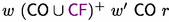 in \(\tau ^r_X\).
 -
3.
For \(X={\texttt {CM}}\), \({\texttt {readable}}(\tau ^r_X, r, x)\) is defined as the set of all write events \(w \in \texttt{E}^{{\textsf{wt}},x}\) s.t. there is no write \(w' \in \texttt{E}^{{\textsf{wt}},x}\) s.t.
 in \(\tau ^r_X\).
 s.t.
s.t.  in
in  in
in Intuitively, \({\texttt {readable}}(\tau ^r_X,r,x)\) contains all write events which are not hidden in \(\tau ^r_X\) by other writes on x. The newly added read event r can fetch its value from a write in \({\texttt {readable}}(\tau ^r_X,r,x)\). The visible set \({\texttt {visible}}(\tau ^r_X, r,x)\) is defined as the set of events in \({\texttt {readable}}(\tau ^r_X,r,x)\) which can “reach” r in \(\tau ^r_X\). Let \(\tau ^{rw}\) denote the trace obtained by adding r and  to trace \(\tau \).
-
1.
For \(X={\texttt {CCv}}\), \({\texttt {visible}}(\tau ^r_X, r,x)=\{e \in {\texttt {readable}}(\tau ^r_X, r,x) \mid e~\textsf{CO}~r\}\). The point of \({\texttt {visible}}(\tau ^r_X, r,x)\) is that when the new read r is added, which reads from a write w, \(\textsf{extend}_X(\tau ^{rw})\) will not contain \(\textsf{Xcycle}\) on adding from each \(e \in {\texttt {visible}}(\tau ^r_X,r,x)\) a
 edge to w. Then \(\textsf{extend}_X(\tau ^{rw})\) contains \(\{(e,w) \mid e \in {\texttt {visible}}(\tau ^r_X, r,x)\}\).
 -
2.
For \(X={\texttt {CM}}\),
 where r is a read in process p. The point of \({\texttt {visible}}(\tau ^r_X, r,x)\) is that when the new read r is added, which reads from a write w, \(\textsf{extend}_X(\tau ^{rw})\) will not contain \(\textsf{Xcycle}\) on adding from each \(e \in {\texttt {visible}}(\tau ^r_X,r,x)\) a
  edge to w. Then \(\textsf{extend}_X(\tau ^{rw})\) contains \(\{(e,w) \mid e \in {\texttt {visible}}(\tau ^r_X, r,x)\}\).
 edge to w. Then
  where r is a read in process p. The point of
  edge to w. Then
 The trace semantics for a model \(X \in \{\texttt{CC}, {\texttt {CCv}}, {\texttt {CM}}\}\) is given as the transition relation \(\xrightarrow []{}_{X{-}{\texttt {tr}}}\), defined as \(\tau _X \xrightarrow []{\alpha }_{X{-}{\texttt {tr}}}\tau '_X\) where \(\textsf{extend}_X(\tau )=\tau _X, \textsf{extend}_X(\tau ')=\tau '_X\). The label \(\alpha \) is one of (read, r, w), (write, w) representing respectively, a read r reading from a write w, and a write event w. An important property of \(\tau _X \xrightarrow []{\alpha }_{X{-}{\texttt {tr}}} \tau '_X\) is that if \(\tau _X\) does not have \(\textsf{Xcycle}\), then \(\tau '_X\) also does not have \(\textsf{Xcycle}\); in other words, if \(\tau \models X\), then \(\tau ' \models X\). We now describe the transitions \(\tau _X\xrightarrow []{\alpha }_{X{-}{\texttt {tr}}} \tau '_X\) where \(\textsf{extend}_X(\tau ) =\tau _X, \textsf{extend}_X(\tau ')=\tau '_X\),  . We start from the empty trace \(\tau _0\), \(\textsf{extend}_X(\tau _0)=\tau _0\).
-
From \(\tau _X\), assume that we observe a write w in process p. In this case, the label \(\alpha \) is (write, w), and we add w, and a
 edge from the
  -latest event of process p in \(\tau _X\) to w obtaining \(\tau '_X\).
 -
From \(\tau _X\), assume we observe a read event r on variable x in process p. In this case, the label \(\alpha \) is (read, r, w), where w is the write from which r reads. Add the read r, a
 edge from the
  -latest event of process p in \(\tau _X\) to r obtaining \(\tau _X^r\). Add
  from a \(w \in {\texttt {readable}}(\tau ^r_X,r,x)\) to r.
-
When \(X={\texttt {CCv}}\). Add new
 edges from all \(w'' \in {\texttt {visible}}(\tau ^r_X, r, x)\) to w to get \(\tau '_X\).
 -
When \(X={\texttt {CM}}\). Add new
 edges from all \(w'' \in {\texttt {visible}}(\tau ^r_X, r, x)\) to w. Adding these
  edges can result in
  for write events \(w_1,w_2\) on a variable y. If we had
  ,
,  , then add
  . When we are done adding all such
  edges, we obtain \(\tau '_X\). (Figure 4(iv)).
-
 edge from the
  -latest event of process p in
  edge from the
  -latest event of process p in
  from a
  edges from all
  edges from all
  edges can result in
  for write events
  ,
,  , then add
  . When we are done adding all such
  edges, we obtain
\(w_1, w_6\) are writes on y, \(r_1\) is a read on y, \(w_2, w_3,w_4, w_5\) are writes on x in \(\tau _{{\texttt {CM}}}\). Add read r on x to \(\tau _{{\texttt {CM}}}\). \(w_2, w_3, w_5 \in {\texttt {readable}}(\tau ^r_{{\texttt {CM}}}, r,x)\). Choose  . Then we add
  and
and  . The addition of
  results in
  . Since
  , add the
  edge from \(r_1\) to \(w_6\) to obtain \(\tau '_{{\texttt {CM}}}\).
Lemma 1
If \(\tau _X=\textsf{extend}_X(\tau )\) with \(\tau \models X\), and \(\tau _X \xrightarrow []{\alpha }_{{\texttt {tr}}} \tau '_X=\textsf{extend}_X(\tau ')\), then \(\tau ' \models X\) for \(X \in \{\texttt{CC}, {\texttt {CCv}}, {\texttt {CM}}\}\).
Efficiency and Correctness. Each step of \(\xrightarrow []{\alpha }_{{\texttt {tr}}}\) is computable in polynomial time . This is based on the fact that readable and visible sets are computable in polynomial time. The correctness of the trace semantics for a model X stems from the fact that it generates only those X-extensions which do not have cycles (Lemma 1). The transitions ensure acyclicity of the resultant extended traces.
5 DPOR Algorithm for \(\texttt{CC}, {\texttt {CCv}}, {\texttt {CM}}\)


We present our DPOR algorithm, which systematically explores, for any terminating program under the consistency models \(X \in \{\texttt{CC}, {\texttt {CCv}}, {\texttt {CM}}\}\), all traces \(\tau _X\) wrt X which can be generated by the trace semantics. Enabled write events from any of the processes are added to the trace generated so far, and we proceed with the next event. For a read event r, we add r to the trace, and explore in separate branches, all possible write events w from which r can read from. Each such branch is a sequence of events also called a schedule. There may be writes \(w'\) which will be added to the trace later in the exploration, from which r can also read. Such writes \(w'\) are called postponed wrt r; when \(w'\) is added to the trace later, the algorithm will have a branch where r can read from \(w'\). In that branch, the algorithm reorders events in the sequence s.t. \(w'\) and r exchange places, and all events which are needed for \(w'\) to occur are also placed before \(w'\) (\(\textsc {CreateSchedule}\)). All generated schedules will be executed by \(\textsc {RunSchedule}\). The algorithm is uniform across the models, with the main technical differences being taken care of by the respective trace semantics which guides the exploration of traces in each model.
The \(\textsc {ExploreTraces}\) Algorithm. This algorithm takes as input, a consistency model \(X \in \{\texttt{CC}, {\texttt {CCv}}, {\texttt {CM}}\}\), an X-extension \(\tau _X\) and an observation sequence \(\pi \). \(\pi \) is a sequence of events of the form (write, w) or (read, r, w). The initial invocation is with the empty trace \(\tau _0\) and observation sequence \(\pi =\epsilon \). The observation sequence is used to swap read operations with write operations that are postponed wrt them. From the initial \(\tau _0\), we choose an operation from any of the processes.
If a write operation is enabled, one such is chosen non deterministically from any process, and is added to the trace according to the trace semantics, and also appended to the observation sequence, whereafter \(\textsc {ExploreTraces}\) is called recursively to continue the exploration (line 3). After the recursive calls have returned, the algorithm calls \(\textsc {CreateSchedule}\), which finds read operations r in the observation sequence which can read from write operations w if w was performed before r. For each such read r, \(\textsc {CreateSchedule}\) creates a schedule for r, an observation sequence that can be explored from the point when r was performed, allowing w to occur before r so that r can read from w. When a read operation r is enabled, the set \(\texttt{Schedules}(r)\) is initialized (line 6). This set is updated by \(\textsc {CreateSchedule}\) when subsequent writes are explored. We also keep a Boolean flag \(\texttt {Swappable}(r)\) for each read event r. This is initialized to true, indicating that r is swappable, that is, subsequent writes can be considered for r. This flag is set to false for read events appearing in a schedule so that they are not swapped, eliminating redundant explorations. For each generated write event w from which r can read, \(\textsc {ExploreTraces}\) is called recursively (line 7)to continue the exploration. Once these recursive calls have returned, the set of schedules collected in \(\texttt{Schedules}(r)\) for the read r is considered. \(\textsc {RunSchedule}\) explores all schedules, where the read fetches its value from the respective write.
The \(\textsc {CreateSchedule}\) algorithm. The input to this algorithm is a consistency model X, a trace \(\tau _X\) wrt X, and an observation sequence \(\pi \) whose last element is a write. The algorithm looks for reads in \(\pi \) for which w is a postponed write. Indeed, this read r and w must be on the same variable, r must be swappable, and r must not precede w wrt \(\textsf{CO}\) (line 4). We begin with the closest (from the write w) such read r at position \(\pi [j]\). After finding r, a schedule \(\beta \) is created. The schedule consists of all elements following r in \(\pi \) and preceding w wrt \(\textsf{CO}\) (line 12). It ends with \(w \bullet (r,w)\), allowing r to read from w (line 13). This schedule is added to \(\texttt{Schedules}(r)\) if it does not already contain a schedule \(\beta '\) which has the same set of observations : \(\texttt{Schedules}(r)\) does not contain \(\beta ' \approx \beta \).
The \(\textsc {RunSchedule}\) Algorithm. The inputs are a consistency model X, a trace \(\tau _X\), an observation sequence \(\pi \) and a schedule \(\beta \). The schedule of observations in \(\beta \) is explored one by one, by recursively calling itself, and updating the trace. The read events in the schedule are not swappable, preventing a redundant exploration for them (schedules where these are swapped with respective writes will be created by \(\textsc {CreateSchedule}\). All proofs and an illustrative example can be found in the extended version of the paper [2].
Theorem 1
Our DPOR algorithms are sound, complete and optimal.
Soundness, Optimality and Completeness. The algorithm is sound in the sense that, if we initiate Algorithm 1 from \((X,\tau _{0},\epsilon )\), then, all explored traces \(\tau \) are s.t. \(\tau \models X\). This follows from the fact that the exploration uses the \(\xrightarrow []{}_{X{-}{\texttt {tr}}}\) relation. The algorithm is optimal in the sense that, for any two different recursive calls to Algorithm 1 with arguments \((X,\tau ^1_X, \pi _1)\) and \((X, \tau ^2_X, \pi _2)\), if \(\tau ^1_X, \tau ^2_X\) are extendible, then \(\tau ^1_X \ne \tau ^2_X\). This follows from (i) for a given read r, each iteration of the for loop in line 7 will correspond to a different write, (ii) in each schedule \(\beta \in \mathtt{{Schedules}}(e)\) in line 8 of Algorithm 1, the read event r reads from a write w which is different from all writes it reads from in line 7 (iii) Any two schedules added to \(\mathtt{{Schedules}}(e)\) at line 14 of Algorithm 2 will be different. The algorithm explores traces of all terminating runs, and is hence complete.
6 Experimental Evaluation
We describe the implementation of our optimal DPOR algorithm for the causal consistency models \(\texttt{CC}, {\texttt {CCv}}, {\texttt {CM}}\) as a tool \(\textsc {Conschecker}\), available at[45]. To the best of our knowledge, Conschecker is the first stateless model checking tool for the causal consistency models \(\texttt{CC}, {\texttt {CCv}}, {\texttt {CM}}\).
Conschecker. Conschecker extends Nidhugg [3] and works at LLVM IR level accepting a C language program as input. At runtime, Conschecker controls the exploration of the input program until it has explored all the traces using the DPOR algorithm. It can detect user-provided assertion violations by analyzing the generated traces. We conduct all experiments on a Ubuntu 22.04.1 LTS with Intel Core i7-1165G7 and 16 GB RAM. We evaluate Conschecker on the following categories of benchmarks, as seen below.
Experimental Setup. We consider the following categories of benchmarks.
-
A set of thousands of litmus tests (sec 6.1) generated from [8]. The main purpose of these experiments is to provide a sanity check of the correctness of Conschecker on all three consistency models.
-
A collection (sec 6.2) of concurrent benchmarks taken from the TACAS competition on software verification [44]. These are small programs with 50-100 lines of code used by many tools [4, 5].
-
Five applications (sec 6.3) : Voter [19], Twitter clone [27], Fusion ticket [27], two versions of Auction [36], extracted from literature on databases, and verify against assertion violations wrt the three consistency models.
-
Classical database benchmarks (sec 6.4) reported in recent papers on consistency models [12, 13] and [14]. We classify these benchmarks SAFE and UNSAFE on all three models depending on whether they witness an assertion violation.
-
Eight parameterized programs (sec 6.5) from [5] and [4] to study the scalability of Conschecker when increasing the number of processes, as well as read and write instructions in programs.
6.1 Litmus Benchmarks
We apply Conschecker on a set of 9815 litmus benchmarks generated from [8]. Litmus tests are standard benchmark programs used by many tools running on weak memories. In these litmus tests, the processes execute concurrently, and we validate assertions on the underlying memory model, doing a sanity check for the correctness of \(\textsc {Conschecker}\). We compared the observed outcomes of \(\textsc {Conschecker}\) on the litmus tests with expected outcomes generated from [8]. We generated the expected outcomes by simulating the \({\texttt {CCv}}\), and \(\texttt{CC}\) and \({\texttt {CM}}\) semantics on [8] for these litmus tests. Out of the 9815 litmus tests, we found no assertion violations in 3810 under \(\texttt{CC}, {\texttt {CM}}\) and 3811 under \({\texttt {CCv}}\). Results obtained from \(\textsc {Conschecker}\) matched with the expected outcomes. \(\textsc {Conschecker}\) took <3 mins to execute on all litmus tests across models.
6.2 SV-COMP Benchmarks
These benchmarks [44] consist of five programs written in C/C++ having 2 processes each, with 50-100 lines of code per process (Table 3). The main challenge in these benchmarks is the large number of traces to be explored. These benchmarks have assertion checks, and under \({\texttt {CCv}}, {\texttt {CM}}\), and \(\texttt{CC}\) all these assertions are violated. \(\textsc {Conschecker}\) stops exploration as soon as it detects the first assertion violation. To check the efficiency of \(\textsc {Conschecker}\), we removed all assertions and let \(\textsc {Conschecker}\) exhaustively explore all  traces. Since these benchmarks have large number of traces, they serve as a stress test.
6.3 Database Applications
Table 2 reports the performance of Conschecker on a set of programs inspired from five applications extracted from the literature on distributed systems [12, 19, 27, 36]. The applications we considered are
-
Voter [19] : This application is derived from a software system used to record votes from a talent show. Users can vote for any of the n contestants from any one of the m sites (processes). The application asserts that users cannot vote from multiple sites and cannot vote for multiple contestants and checks for violations of this. [19] considers 3 sites and 3 users, and we follow suit.
-
Twitter clone [27] : This is based on a twitter like service where each user has some followers. The following assertion is checked : when the user tweets, the tweet ID must be added to the follower’s time line exactly once if the user did not remove his tweet. We considered 3 users using 3 processes, each process has 10 tweet IDs and 6 followers.
-
Fusion ticket [27] : There is a building having multiple concert rooms (venues). Tickets for venue i are sold by salesperson i who updates in the backend database, the sales for the day. The per venue ticket sale must be updated correctly in the database, so that the concert manager sees the correct total number of tickets sold. A discrepancy in this number is a violation. Each venue is represented by a process, and the communication across processes ensures the total sum is correct. We considered 4 venues and each venue had 10 tickets.
-
Auction [36] and Auction-2 [36]: There are n bidders and an auctioneer participating in an auction, modeled using \(n+1\) processes. The assertion to be checked is that the highest bidder must be declared winner. Auction is the buggy version for this application, while Auction-2 is the correct one.
-
Group is a synthetic application created by us inspired from whatsapp groups. There is a group with n members, and a new person wants to be added to the group. This person must be added to the group only by one of the existing members. That is, a violation constitutes to adding a person more than once (by one or more members). We check with 6 processes(members).
6.4 Classical Benchmarks
Table 1 consists of classical benchmarks [12,13,14] and [11] which test for some assertion violations under the three models. Since the traces generated differ for each model \(X \in \{\texttt{CC}, {\texttt {CCv}}, {\texttt {CM}}\}\), the violations also differ. For the ones marked SAFE under model \(X \in \{\texttt{CC}, {\texttt {CCv}}, {\texttt {CM}}\}\), the assertion violation did not occur under any execution, while the unsafe ones reported the violation. We consider twenty such examples. We consider three different versions of each example, varying the number of processes and variables.
For each example, we have three versions by parameterizing the number of processes and instructions. In version 1, we have four processes per program and three to five instructions per process. Version 2 is obtained allowing each process to have seven-ten instructions. Version 3 expands version 2 by allowing each program to have up to five-six processes and up to 15-20 instructions. The number of instructions is increased by introducing fresh variables and having reads/writes on them. Versions 2,3 serve as a stress test for Conschecker as increasing the number of instructions and processes increases the number of of consistent traces. Conschecker took less than 3s to finish running all version 1 programs, about 30s to finish running all version 2 programs and about 200s to finish running all version 3 programs.
6.5 Parameterized Benchmarks
Table 4 reports experimental results of Conschecker on 8 parameterized benchmarks. Out of these, in redundant-co(N) (taken from [5]), N is the number of loop iterations per process in a program with 3 processes. In all others, the parameterization is on the number of processes. This set of benchmarks serves to check the scalability of Conschecker. As seen in Table 4, Conschecker scales up to 20 processes (n-writers-a-read) and 13 variables (lastzero).
7 Conclusion
In this paper, we have provided a DPOR algorithm using the  equivalence for three prominent causal consistency models, and also implemented the same in a tool Conschecker. This is the first tool for stateless model checking of causal consistency models. We plan to extend our work by develo** a DPOR algorithm for transactional programs under \(\texttt{CC}, {\texttt {CCv}}, {\texttt {CM}}\) [12]. For these, the extra complication is the presence of transactions which must be executed atomically without interference in each process. The final notch is to handle snapshot isolation, the strongest among transactional consistency models.
8 Data-Availability Statement
The tool and experimental data for the study are available at the Zenodo repository: [45].
References
Abdulla, P., Aronis, S., Jonsson, B., Sagonas, K.: Optimal dynamic partial order reduction. SIGPLAN Not. 49(1), 373–384 (jan 2014). https://doi.org/10.1145/2578855.2535845, https://doi.org/10.1145/2578855.2535845
Abdulla, P., Atig, M.F., S, K., Gupta, A., Tuppe, O.: Optimal Stateless Model Checking for Causal Consistency (Jan 2023). https://doi.org/10.5281/zenodo.7572282, https://doi.org/10.5281/zenodo.7572282
Abdulla, P.A., Aronis, S., Atig, M.F., Jonsson, B., Leonardsson, C., Sagonas, K.: Stateless model checking for tso and pso. In: Baier, C., Tinelli, C. (eds.) Tools and Algorithms for the Construction and Analysis of Systems. pp. 353–367. Springer Berlin Heidelberg, Berlin, Heidelberg (2015)
Abdulla, P.A., Atig, M.F., Jonsson, B., Lång, M., Ngo, T.P., Sagonas, K.: Optimal stateless model checking for reads-from equivalence under sequential consistency. Proc. ACM Program. Lang. 3(OOPSLA) (Oct 2019). https://doi.org/10.1145/3360576, https://doi.org/10.1145/3360576
Abdulla, P.A., Atig, M.F., Jonsson, B., Ngo, T.P.: Optimal stateless model checking under the release-acquire semantics. Proc. ACM Program. Lang. 2(OOPSLA) (Oct 2018). https://doi.org/10.1145/3276505, https://doi.org/10.1145/3276505
Agarwal, P., Chatterjee, K., Pathak, S., Pavlogiannis, A., Toman, V.: Stateless model checking under a reads-value-from equivalence. In: Silva and Leino [43], pp. 341–366. https://doi.org/10.1007/978-3-030-81685-8_16, https://doi.org/10.1007/978-3-030-81685-8_16
Ahamad, M., Neiger, G., Burns, J.E., Kohli, P., Hutto, P.W.: Causal memory: Definitions, implementation, and programming. Distrib. Comput. 9(1), 37–49 (Mar 1995). https://doi.org/10.1007/BF01784241, https://doi.org/10.1007/BF01784241
Alglave, J., Maranget, L., Tautschnig, M.: Herding cats: Modelling, simulation, testing, and data mining for weak memory. ACM Trans. Program. Lang. Syst. 36(2) (jul 2014). https://doi.org/10.1145/2627752, https://doi.org/10.1145/2627752
Bailis, P., Ghodsi, A., Hellerstein, J.M., Stoica, I.: Bolt-on causal consistency. In: Ross, K.A., Srivastava, D., Papadias, D. (eds.) Proceedings of the ACM SIGMOD International Conference on Management of Data, SIGMOD 2013, New York, NY, USA, June 22-27, 2013. pp. 761–772. ACM (2013). https://doi.org/10.1145/2463676.2465279, https://doi.org/10.1145/2463676.2465279
Batty, M., Owens, S., Sarkar, S., Sewell, P., Weber, T.: Mathematizing C++ concurrency. In: Ball, T., Sagiv, M. (eds.) Proceedings of the 38th ACM SIGPLAN-SIGACT Symposium on Principles of Programming Languages, POPL 2011, Austin, TX, USA, January 26-28, 2011. pp. 55–66. ACM (2011). https://doi.org/10.1145/1926385.1926394, https://doi.org/10.1145/1926385.1926394
Beillahi, S.M., Bouajjani, A., Enea, C.: Checking robustness between weak transactional consistency models. Programming Languages and Systems 12648, 87 (2021)
Beillahi, S.M., Bouajjani, A., Enea, C.: Robustness Against Transactional Causal Consistency. Logical Methods in Computer Science Volume 17, Issue 1 (Feb 2021). https://doi.org/10.23638/LMCS-17(1:12)2021, https://lmcs.episciences.org/7149
Bernardi, G., Gotsman, A.: Robustness against consistency models with atomic visibility. In: 27th International Conference on Concurrency Theory (CONCUR 2016). Schloss Dagstuhl-Leibniz-Zentrum fuer Informatik (2016)
Biswas, R., Enea, C.: On the complexity of checking transactional consistency. Proc. ACM Program. Lang. 3(OOPSLA) (oct 2019). https://doi.org/10.1145/3360591, https://doi.org/10.1145/3360591
Bouajjani, A., Enea, C., Guerraoui, R., Hamza, J.: On verifying causal consistency. In: Proceedings of the 44th ACM SIGPLAN Symposium on Principles of Programming Languages. p. 626–638. POPL 2017, Association for Computing Machinery, New York, NY, USA (2017). https://doi.org/10.1145/3009837.3009888, https://doi.org/10.1145/3009837.3009888
Burckhardt, S.: Principles of eventual consistency. Found. Trends Program. Lang. 1(1-2), 1–150 (2014). https://doi.org/10.1561/2500000011, https://doi.org/10.1561/2500000011
Christakis, M., Gotovos, A., Sagonas, K.: Systematic testing for detecting concurrency errors in erlang programs. In: Sixth IEEE International Conference on Software Testing, Verification and Validation, ICST 2013, Luxembourg, Luxembourg, March 18-22, 2013. pp. 154–163. IEEE Computer Society (2013). https://doi.org/10.1109/ICST.2013.50, https://doi.org/10.1109/ICST.2013.50
Clarke, E.M., Grumberg, O., Minea, M., Peled, D.A.: State space reduction using partial order techniques. Int. J. Softw. Tools Technol. Transf. 2(3), 279–287 (1999). https://doi.org/10.1007/s100090050035, https://doi.org/10.1007/s100090050035
Difallah, D.E., Pavlo, A., Curino, C., Cudre-Mauroux, P.: Oltp-bench: An extensible testbed for benchmarking relational databases. Proc. VLDB Endow. 7(4), 277–288 (dec 2013). https://doi.org/10.14778/2732240.2732246, https://doi.org/10.14778/2732240.2732246
Du, J., Elnikety, S., Roy, A., Zwaenepoel, W.: Orbe: scalable causal consistency using dependency matrices and physical clocks. In: Lohman, G.M. (ed.) ACM Symposium on Cloud Computing, SOCC ’13, Santa Clara, CA, USA, October 1-3, 2013. pp. 11:1–11:14. ACM (2013). https://doi.org/10.1145/2523616.2523628, https://doi.org/10.1145/2523616.2523628
Du, J., Iorgulescu, C., Roy, A., Zwaenepoel, W.: Gentlerain: Cheap and scalable causal consistency with physical clocks. In: Lazowska, E., Terry, D., Arpaci-Dusseau, R.H., Gehrke, J. (eds.) Proceedings of the ACM Symposium on Cloud Computing, Seattle, WA, USA, November 3-5, 2014. pp. 4:1–4:13. ACM (2014). https://doi.org/10.1145/2670979.2670983, https://doi.org/10.1145/2670979.2670983
Godefroid, P.: Partial-Order Methods for the Verification of Concurrent Systems - An Approach to the State-Explosion Problem, Lecture Notes in Computer Science, vol. 1032. Springer (1996). https://doi.org/10.1007/3-540-60761-7, https://doi.org/10.1007/3-540-60761-7
Godefroid, P.: Model checking for programming languages using verisoft. In: Proceedings of the 24th ACM SIGPLAN-SIGACT Symposium on Principles of Programming Languages. p. 174–186. POPL ’97, Association for Computing Machinery, New York, NY, USA (1997). https://doi.org/10.1145/263699.263717, https://doi.org/10.1145/263699.263717
Godefroid, P.: Software model checking: The verisoft approach. Form. Methods Syst. Des. 26(2), 77–101 (Mar 2005). https://doi.org/10.1007/s10703-005-1489-x, https://doi.org/10.1007/s10703-005-1489-x
Hamza, J.: Algorithmic Verification of Concurrent and Distributed Data Structures. Ph.D. thesis, Université Paris Diderot (2015)
Herlihy, M., Wing, J.M.: Linearizability: A correctness condition for concurrent objects. ACM Trans. Program. Lang. Syst. 12(3), 463–492 (1990). https://doi.org/10.1145/78969.78972, https://doi.org/10.1145/78969.78972
Holt, B., Bornholt, J., Zhang, I., Ports, D., Oskin, M., Ceze, L.: Disciplined inconsistency with consistency types. In: Proceedings of the Seventh ACM Symposium on Cloud Computing. p. 279–293. SoCC ’16, Association for Computing Machinery, New York, NY, USA (2016). https://doi.org/10.1145/2987550.2987559, https://doi.org/10.1145/2987550.2987559
Kokologiannakis, M., Lahav, O., Sagonas, K., Vafeiadis, V.: Effective stateless model checking for C/C++ concurrency. Proc. ACM Program. Lang. 2(POPL), 17:1–17:32 (2018). https://doi.org/10.1145/3158105, https://doi.org/10.1145/3158105
Kokologiannakis, M., Marmanis, I., Gladstein, V., Vafeiadis, V.: Truly stateless, optimal dynamic partial order reduction. Proc. ACM Program. Lang. 6(POPL), 1–28 (2022). https://doi.org/10.1145/3498711, https://doi.org/10.1145/3498711
Kokologiannakis, M., Vafeiadis, V.: Genmc: A model checker for weak memory models. In: Silva, A., Leino, K.R.M. (eds.) Computer Aided Verification. pp. 427–440. Springer International Publishing, Cham (2021)
Lahav, O.: Verification under causally consistent shared memory. ACM SIGLOG News 6(2), 43–56 (2019). https://doi.org/10.1145/3326938.3326942, https://doi.org/10.1145/3326938.3326942
Lamport, L.: Time, clocks, and the ordering of events in a distributed system. Commun. ACM 21(7), 558–565 (1978). https://doi.org/10.1145/359545.359563, https://doi.org/10.1145/359545.359563
Lamport, L.: How to make a multiprocessor computer that correctly executes multiprocess programs. IEEE Trans. Computers 28(9), 690–691 (1979). https://doi.org/10.1109/TC.1979.1675439, https://doi.org/10.1109/TC.1979.1675439
Mazurkiewicz, A.: Trace theory. In: Advances in Petri Nets 1986, Part II on Petri Nets: Applications and Relationships to Other Models of Concurrency. p. 279–324. Springer-Verlag, Berlin, Heidelberg (1987)
Musuvathi, M., Qadeer, S., Ball, T., Basler, G., Nainar, P.A., Neamtiu, I.: Finding and reproducing heisenbugs in concurrent programs. In: Draves, R., van Renesse, R. (eds.) 8th USENIX Symposium on Operating Systems Design and Implementation, OSDI 2008, December 8-10, 2008, San Diego, California, USA, Proceedings. pp. 267–280. USENIX Association (2008), http://www.usenix.org/events/osdi08/tech/full_papers/musuvathi/musuvathi.pdf
Nair, S.S., Petri, G., Shapiro, M.: Proving the safety of highly-available distributed objects. In: Müller, P. (ed.) Programming Languages and Systems. pp. 544–571. Springer International Publishing, Cham (2020)
Norris, B., Demsky, B.: A practical approach for model checking c/c++11 code. ACM Trans. Program. Lang. Syst. 38(3) (May 2016). https://doi.org/10.1145/2806886, https://doi.org/10.1145/2806886
Owens, S., Sarkar, S., Sewell, P.: A better x86 memory model: x86-tso. In: Berghofer, S., Nipkow, T., Urban, C., Wenzel, M. (eds.) Theorem Proving in Higher Order Logics, 22nd International Conference, TPHOLs 2009, Munich, Germany, August 17-20, 2009. Proceedings. Lecture Notes in Computer Science, vol. 5674, pp. 391–407. Springer (2009). https://doi.org/10.1007/978-3-642-03359-9_27, https://doi.org/10.1007/978-3-642-03359-9_27
Perrin, M., Mostéfaoui, A., Jard, C.: Causal consistency: beyond memory. In: Asenjo, R., Harris, T. (eds.) Proceedings of the 21st ACM SIGPLAN Symposium on Principles and Practice of Parallel Programming, PPoPP 2016, Barcelona, Spain, March 12-16, 2016. pp. 26:1–26:12. ACM (2016). https://doi.org/10.1145/2851141.2851170, https://doi.org/10.1145/2851141.2851170
Raynal, M., Schiper, A.: From causal consistency to sequential consistency in shared memory systems. In: Thiagarajan, P.S. (ed.) Foundations of Software Technology and Theoretical Computer Science, 15th Conference, Bangalore, India, December 18-20, 1995, Proceedings. Lecture Notes in Computer Science, vol. 1026, pp. 180–194. Springer (1995). https://doi.org/10.1007/3-540-60692-0_48, https://doi.org/10.1007/3-540-60692-0_48
Sen, K., Agha, G.: A race-detection and flip** algorithm for automated testing of multi-threaded programs. In: Proceedings of the 2nd International Haifa Verification Conference on Hardware and Software, Verification and Testing. p. 166–182. HVC’06, Springer-Verlag, Berlin, Heidelberg (2006)
Shasha, D.E., Snir, M.: Efficient and correct execution of parallel programs that share memory. ACM Trans. Program. Lang. Syst. 10(2), 282–312 (1988). https://doi.org/10.1145/42190.42277, https://doi.org/10.1145/42190.42277
Silva, A., Leino, K.R.M. (eds.): Computer Aided Verification - 33rd International Conference, CAV 2021, Virtual Event, July 20-23, 2021, Proceedings, Part I, Lecture Notes in Computer Science, vol. 12759. Springer (2021). https://doi.org/10.1007/978-3-030-81685-8, https://doi.org/10.1007/978-3-030-81685-8
SV-COMP: Competition on Software Verification. https://sv-comp.sosy-lab.org/2018 (2018), [Online; accessed 2017-11-10]
Tuppe, O.: Conschecker (Jan 2023). https://doi.org/10.5281/zenodo.7500551, https://doi.org/10.5281/zenodo.7500551
Zhang, N., Kusano, M., Wang, C.: Dynamic partial order reduction for relaxed memory models. In: Proceedings of the 36th ACM SIGPLAN Conference on Programming Language Design and Implementation. p. 250–259. PLDI ’15, Association for Computing Machinery, New York, NY, USA (2015). https://doi.org/10.1145/2737924.2737956, https://doi.org/10.1145/2737924.2737956
Author information
Authors and Affiliations
Corresponding author
Editor information
Editors and Affiliations
Rights and permissions
Open Access This chapter is licensed under the terms of the Creative Commons Attribution 4.0 International License (http://creativecommons.org/licenses/by/4.0/), which permits use, sharing, adaptation, distribution and reproduction in any medium or format, as long as you give appropriate credit to the original author(s) and the source, provide a link to the Creative Commons license and indicate if changes were made.
The images or other third party material in this chapter are included in the chapter's Creative Commons license, unless indicated otherwise in a credit line to the material. If material is not included in the chapter's Creative Commons license and your intended use is not permitted by statutory regulation or exceeds the permitted use, you will need to obtain permission directly from the copyright holder.
Copyright information
© 2023 The Author(s)
About this paper

Cite this paper
Abdulla, P., Atig, M.F., Krishna, S., Gupta, A., Tuppe, O. (2023). Optimal Stateless Model Checking for Causal Consistency. In: Sankaranarayanan, S., Sharygina, N. (eds) Tools and Algorithms for the Construction and Analysis of Systems. TACAS 2023. Lecture Notes in Computer Science, vol 13993. Springer, Cham. https://doi.org/10.1007/978-3-031-30823-9_6
Download citation
DOI: https://doi.org/10.1007/978-3-031-30823-9_6
Published:
Publisher Name: Springer, Cham
Print ISBN: 978-3-031-30822-2
Online ISBN: 978-3-031-30823-9
eBook Packages: Computer ScienceComputer Science (R0)