Singular Integral Equations

Abstract

The construction of exact solutions for radiative transfer equations is always based on the transformation of these equations into new ones, for which exact methods of solutions have been developed, in other branches of physics or in mathematical physics. For infinite media, as shown in Sect. 3.1, the integral equation for the source function can be transformed into an algebraic equation by performing a Fourier transform. For radiative transfer problems in a semi-infinite medium, the situation is not as simple, but they can be transformed into singular integral equations with Cauchy-type kernels for which powerful methods of solutions have been developed, such as the Hilbert transform method introduced by T. Carlemann in 1922. In this Chapter, we show how to transform a Wiener–Hopf integral equation into a singular integral equation. We present two different methods, using the equation for S(τ) as example. We then present the main lines of the Hilbert transform method of solution, which will be applied to scalar as well as to polarized radiative transfer problems. A third method leading to a singular integral equation is described in Chap. 10. It is based on a singular eigenfunction expansion of the radiation field, introduced by K. Case in 1960.

Appendices

Appendix A: Hilbert Transforms

A.1 Definition and Properties

The Hilbert transform $\mathcal {F}(z)$ of a function f(u) is defined by

$$\displaystyle \begin{aligned} \mathcal{F}(z)\equiv \frac{1}{2\mathrm{i}\,\uppi}\int_L \frac{f(u)}{u -z}\,du, {} \end{aligned} $$

(A.1)

where L is a line in the complex plane, z a point in the complex plane, not belonging to L and f(u) a complex-valued function defined on L. The line L can be an arc or a closed contour. The integral in Eq. (A.1) is a Cauchy integral. These integrals are well known to mathematicians and their properties have been studied in great detail by Muskhelishvili (1953), when f(u) is a Hölder continuous function. Cauchy integrals are treated in detail in many textbooks dealing with functions of a complex variable, such as Gakhov (1966), Pogorzelski (1966), Carrier et al. (1966), Roos (1969), Dautray and Lions (1984, vol. 6), Ablowitz and Fokas (1997) and also in books devoted to transport theory, such as Noble (1958), Case and Zweifel (1967), Duderstadt and Martin (1979), to name only a few.

We recall here some properties that are in frequent use in this book.

• $\mathcal {F}(z)$ is analytic⁴ in the complex plane cut along the line L. The existence of a cut implies that $\mathcal {F}(z)$ has different values on each side of the cut, say $\mathcal {F}^+(u)$ and $\mathcal {F}^-(u)$ and to go from one side of the cut to the other, it is necessary to circulate around the cut.

• The limiting values, $\mathcal {F}^ +(u)$ and $\mathcal {F}^ -(u)$ satisfy the Plemelj formulae (also called the Sokhotskii–Plemelj formulae). They state that

  $$\displaystyle \begin{aligned} \begin{array}{rcl} \mathcal{F}^+(u) - \mathcal{F}^-(u)& =&\displaystyle f(u), {} \end{array} \end{aligned} $$

  (A.2)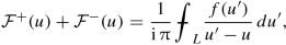
  

  (A.3)

  where means that the integral is taken in Cauchy Principal Value. Here, L will in general be an interval on the real axis, oriented from −∞ to + ∞. Then $\mathcal {F}^+(u)$ is the limit from above, while $\mathcal {F}^-(u)$ is the limit from below, that is

  $$\displaystyle \begin{aligned} \mathcal{F}^\pm(u)\equiv\lim_{\eta\to0}\mathcal{F}(u\pm \mathrm{i}\,\eta),\quad u\mbox{ and }\eta\mbox{ real},\quad \eta>0. {} \end{aligned} $$

  (A.4)

  For an arbitrary arc L, the limiting values are defined with respect to the outside and the inside of a closed oriented contour including the arc L. A simplified derivation of Plemelj formulae is presented in Sect. A.2 and a verification that they hold also when f(u) is a Dirac distribution in Sect. A.3.

• $\mathcal {F}(z)$ tends to zero at infinity. How fast it tends to zero depends on L and f(u). For instance, when f(u) is integrable, $\mathcal {F}(z)$ tends to zero as 1∕z. When the integral of f(u) is zero, then $\mathcal {F}(z)$ tends to zero as 1∕z ².

• $\mathcal {F}(z)$ has a mild (integrable) singularity at the end point(s) of L. This means that for a point z in the neighborhood of the extremity a of the curve L, but not on L, we have

  $$\displaystyle \begin{aligned} |\mathcal{F}(z)|\le C/|z-a|{}^\alpha,\quad 0\le\alpha<1, {} \end{aligned} $$

  (A.5)

  where C is a constant. When f(a) has a non zero value, then $\mathcal {F}(z)$ has a logarithmic singularity, which does satisfy this condition.

A.2 The Plemelj Formulae

Rigorous proofs can be found in most of the references listed above. Carrier et al. (1966) is recommended. Here we give only the main lines of the proof. Also to simplify we assume that L is an interval [a, b] on the real axis and that f(u) is real.

We consider a point z above the real axis approaching the point u on the line L. We assume that f(z) is analytic at the point u and deform the integration line L, as shown in Fig. A.1. We denote by ρ the radius of the half-circle centered on u, lying below the real axis. Along this contour, Eq. (A.1) becomes

$$\displaystyle \begin{aligned} \begin{array}{rcl} {} & &\displaystyle {\mathcal{F}(z)=\frac{1}{2\mathrm{i}\,\uppi}\left[\int_a^{u-\rho} \frac{f(u')}{ u'-z}\,du' + \int_{u+\rho}^b \frac{f(u')}{u'-z}\,du' \right.} \\ & &\displaystyle \ \ + \left. \int_\uppi^{2\uppi} \frac{f(u+ \rho \mathrm{e}^{\mathrm{i}\,\theta})}{u +\rho \mathrm{e}^{\mathrm{i}\,\theta}-z} \rho \mathrm{e}^{\mathrm{i}\,\theta} \mathrm{i}\,\,d\theta\right]. \end{array} \end{aligned} $$

(A.6)

Letting z → u and ρ → 0, replacing f(u + ρe^{i θ}) by f(u) in the last integral, and performing the integration over θ, we obtain

(A.7)

We stress that the integral over [a, b] is a Principal Value integral.

Fig. A.1

Integration contour for the Plemelj formulae. The contribution from the singular point is obtained by letting ρ → 0

We now consider a point z lying below L and deform the integration line as shown in Fig. A.1. The half-circle lies above the real axis. Proceeding exactly as above, we obtain

(A.8)

The negative sign in the first term comes from the variation of θ from π to 0. Combining Eqs. (A.7) and (A.8), we obtain the Plemelj formulae (A.2) and (A.3).

A.3 The Plemelj Formulae for a Dirac Distribution

Although the Dirac distribution δ is not a Hölder continuous function, one can still define a Hilbert transform and establish the Plemelj formulae. The subject of Hilbert transform for Schwartz distributions in treated in Pandey (1996). Here we give the example of the Dirac distribution.

We consider

$$\displaystyle \begin{aligned} \mathcal{F}(z)= \frac{1}{2\mathrm{i}\,\uppi}\int_a^b \frac{\delta(u)}{u-z}\,du. \end{aligned} $$

(A.9)

We assume that the interval [a, b] contains the origin. We consider a point z = u + i 𝜖, 𝜖 > 0 (located above [a, b]). We have

$$\displaystyle \begin{aligned} \mathcal{F}(u+\mathrm{i}\,\epsilon)= \frac{1}{2\mathrm{i}\,\uppi}\int_a^b \frac{\delta(u')}{ u'-(u+\mathrm{i}\,\epsilon)}\,du'= -\frac{1}{2\mathrm{i}\,\uppi}\frac{1}{u +\mathrm{i}\, \epsilon}. \end{aligned} $$

(A.10)

Similarly, for a point z = u −i 𝜖, located below the interval [a, b] we have

$$\displaystyle \begin{aligned} \mathcal{F}(u-\mathrm{i}\,\epsilon)= \frac{1}{2i\uppi}\int_a^b \frac{\delta(u')}{ u'-(u-\mathrm{i}\,\epsilon)}\,du'= -\frac{1}{2\mathrm{i}\,\uppi}\frac{1}{u -\mathrm{i}\, \epsilon}. \end{aligned} $$

(A.11)

Thus

$$\displaystyle \begin{aligned} \begin{array}{rcl} \mathcal{F}(u+\mathrm{i}\,\epsilon) - \mathcal{F}(u-\mathrm{i}\,\epsilon)& =&\displaystyle \frac{1}{ \uppi}\frac{\epsilon}{u^2 + \epsilon^2} {} \end{array} \end{aligned} $$

(A.12)

$$\displaystyle \begin{aligned} \begin{array}{rcl} \mathcal{F}(u+\mathrm{i}\,\epsilon) +\mathcal{F}(u-\mathrm{i}\,\epsilon)& =&\displaystyle - \frac{1}{\mathrm{i}\,\uppi}\frac {u}{u^2 + \epsilon^2}. {} \end{array} \end{aligned} $$

(A.13)

In the limit 𝜖 → 0, the right-hand side in Eq. (A.12) tends to the Dirac distribution and the right-hand side in Eq. (A.13) to − (1∕i π)(P∕u), where P stands for the Cauchy Principal Value. Hence, we obtain

$$\displaystyle \begin{aligned} \begin{array}{rcl} \mathcal{F}^+(u) - \mathcal{F}^-(u)& =&\displaystyle \delta(u) {} \end{array} \end{aligned} $$

(A.14)

$$\displaystyle \begin{aligned} \begin{array}{rcl} \mathcal{F}^+(u) + \mathcal{F}^-(u)& =&\displaystyle - \frac{1}{\mathrm{i}\,\uppi}\frac{P}{u}. {} \end{array} \end{aligned} $$

(A.15)

We can rewrite these equations as

$$\displaystyle \begin{aligned} \mathcal{F}^+(u)= \frac{1}{2}[\delta(u) -\frac{1}{\mathrm{i}\,\uppi}\frac{P}{u}]\equiv \delta^-(u), {} \end{aligned} $$

(A.16)

$$\displaystyle \begin{aligned} -\mathcal{F}^-(u)= \frac{1}{2}[\delta(u) +\frac{1}{\mathrm{i}\,\uppi}\frac{P}{ u}]\equiv\delta^+(u). {} \end{aligned} $$

(A.17)

The distributions δ ⁺ and δ ⁻ are defined in such a way that δ ⁺ + δ ⁻ = δ. They are of frequent use in Quantum Mechanics. They are related to the Fourier transforms $\widehat Y(k)$ and $\widehat Y_{-}(k)$ of the Heaviside function Y (x) and Y ₋(x) ≡ Y (−x). Using

$$\displaystyle \begin{aligned} \lim_{\epsilon\to 0}\hat Y(k +\mathrm{i}\,\epsilon)=\int_0^\infty \mathrm{e}^{\mathrm{i}\,(k+\mathrm{i}\,\epsilon)x}\,dx,\quad k\ \mbox{real},\quad \epsilon>0, {} \end{aligned} $$

(A.18)

and a similar definition for $\widehat Y_{-}(k)$, we obtain

$$\displaystyle \begin{aligned} \widehat Y(k)= 2\uppi \delta^-(k),\quad \widehat Y_{-}(k)= 2\uppi \delta^+(k). {} \end{aligned} $$

(A.19)

References

Ablowitz, M.J., Fokas, A.S.: Complex Variables, Introduction and Applications. Cambridge University Press, Cambridge (1997)
Carleman, T.: Sur la résolution de certaines équations intégrales. Ark. Mat. Astr. Fys. 16, 1–19 (1922)
Carrier, G.F., Krook, M., Pearson, C.E.: Functions of a Complex Variable. McGraw-Hill Book Company, New York (1966)
Case, K.M.: Elementary solutions of the transport equation and their applications. Ann. Phys. (New York) 9, 1–23 (1960)
Case, K.M., Zweifel, P.: Linear Transport Theory. Addison-Wesley, Reading, MA (1967)
Dautray, R., Lions, J.-L.: Analyse Mathématique et calcul numérique pour les sciences et les techniques. Masson, Paris (1984); 1984–1985 (3 Vols.); 1988 (9 Vols.); English edition: Mathematical Analysis and Numerical Methods for Science and Technology (6 Vols.). Springer, Berlin (1990)
Duderstadt, J.J., Martin, W.R.: Transport Theory. Wiley, New York (1979)
Estrada, R., Kanwal, R.P.: The Carleman type singular integral equations. SIAM Rev. 29, 263–290 (1987)
Frisch, H.: A Cauchy integral equation method for analytic solutions of half-space convolution equations. J. Quant. Spectrosc. Radiat. Transf. 39, 149–162 (1988b)
Frisch, H., Frisch, U.: A method of Cauchy integral equation for non-coherent transfer in half-space. J. Quant. Spectrosc. Radiat. Transf. 28, 361–375 (1982)
Frisch, H., van der Mee, C.V., Zweifel, P.: Distributional solutions of singular integral equations. J. Integral Equa. Appl. 2, 205–210 (1990)
Gakhov, F.D.: Boundary Value Problems. Pergamon Press, London (1966); translation by I.N. Sneddon of the 2nd Russian edition (1963). Fizmatgiz, Moscow
Halpern, O., Lueneburg, R., Clark, O.: On multiple scattering of neutrons I. Theory of the albedo of a plane boundary. Phys. Rev. 53, 173–183 (1938)
Kourganoff, V.: Basic Methods in Transfer Problems. Radiative Equilibrium and Neutron Diffusion. Dover Publications, New York (1963); First edition: Oxford University Press, London (1952)
Mc Cormick, N.J., Kuščer, I.: Singular eigenfunction expansions in neutron transport theory. In: Henley, E.J., Lewins, J. (eds.) Advances in Nuclear Science and Technology, vol. 7, pp. 181–282. Academic Press, New York (1973)
Muskhelishvili, N.I.: Singular Integral Equations, Noordhoff, Groningen (based on the second Russian edition published in 1946) (1953); Dover Publications (1991)
Noble, B.: Methods Based on the Wiener–Hopf Technique for the Solution of Partial Differential Equations. Pergamon Press, New York (1958)
Pandey, J.N.: The Hilbert Transform of Schwartz Distributions and Applications. Wiley Inc., New York (1996)
Pogorzelski, W.: Integral Equations and their Applications. Pergamon Press, New York (1966)
Roos, B.W.: Analytic Functions and Distributions in Physics and Engineering. Wiley, New York (1969)
Van der Mee, C.V.M., Zweifel, P.F.: Application of orthogonality relations to singular integral equations. J. Integral Equa. Appl. 2, 185–203 (1990)
Author information
Authors and Affiliations