
Abstract
Effectively sampling and analyzing wetland vegetation is an important part of wetland science, as an indicator of wetland health and quality, and jurisdictional and mitigation success determinations. This chapter explains spatiotemporal vegetation sampling considerations by addressing key questions, such as which wetlands should be sampled and when and at what scale sampling should occur. It also plainly discusses the advantages and disadvantages of basic sampling techniques, such as different types of plot-based, plotless, and relevé systems. Methods of assessing different vegetation and environmental attributes, such as cover and functional groups are discussed in detail. The chapter then describes methods of analyzing wetland vegetation, including simple summary analyses and more complex multivariate methods, such as classification, ordination, and floristic quality indices. Explanations of different types of these analyses and their advantages and disadvantages are provided. Finally, both field and laboratory-based exercises in sampling and analysis are provided for faculty and students studying wetland vegetation.
Access this chapter
Tax calculation will be finalised at checkout
Purchases are for personal use only
References
Allen TFH, Wyleto EP (1983) A hierarchical model for the complexity of plant-communities. J Theor Biol 101:529–540
Andreas BK, Mack JJ, McCormac JS (2004) Floristic Quality Assessment Index (FQAI) for vascular plants and mosses for the State of Ohio. Ohio Environmental Protection Agency, Division of Surface Water, Wetland Ecology Group, Columbus
Atkinson RB, Perry JE, Smith E, Cairns J (1993) Use of created wetland delineation and weighted averages as a component of assessment. Wetlands 13:185–193
Barbour MG, Burk JH, Pitts WD, Gilliam FS, Schwartz MW (1998) Terrestrial plant ecology. Benjamin Cummings, Menlo Park
Bedford BL, Walbridge MR, Aldous A (1999) Patterns in nutrient availability and plant diversity of temperate North American wetlands. Ecology 80:2151–2169
Bonham CD (1989) Measurements for terrestrial vegetation. Wiley, New York
Bouchard V, Frey SD, Gilbert JM, Reed SE (2007) Effects of macrophyte functional group richness on emergent freshwater wetland functions. Ecology 88:2903–2914
Braun-Blanquet MM (1965) Plant sociology: the study of plant communities. Hafner, London
Brinson MM (1993) A hydrogeomorphic classification for wetlands. WRP-DE-4. U.S. Army Corps of Engineers Waterways Experiment Station, Vicksburg
Carr SC, Robertson KM, Peet RK (2010) A vegetation classification of fire-dependent pinelands of Florida. Castanea 75:153–189
Cohen MJ, Lane CR, Reiss KC, Surdick JA, Bardi E, Brown MT (2005) Vegetation based classification trees for rapid assessment of isolated wetland condition. Ecol Indic 5:189–206
Colwell RK (2009) EstimateS: statistical estimation of species richness and shared species from samples 8.2. http://purl.oclc.org/estimates
Curtis JT (1959) The vegetation of Wisconsin: an ordination of plant communities. University of Wisconsin Press, Madison
Dale MRT (1998) Spatial pattern analysis in plant ecology. Cambridge University Press, New York
Daubenmire RF (1959) A canopy coverage method of vegetational analysis. Northwest Sci 33:43–64
De’ath G, Fabricius KE (2000) Classification and regression trees: a powerful yet simple technique for ecological data analysis. Ecology 81:3178–3192
Dufrêne M, Legendre P (1997) Species assemblages and indicator species: the need for a flexible asymmetrical approach. Ecol Monogr 67:345–366
Ehrenfeld JG (1995) Microtopography and vegetation in Atlantic white cedar swamps: the effects of natural disturbances. Can J Bot 73:474–484
Elzinga CL, Salzer DW, Willoughby JW (1998) Measuring and monitoring plant populations. 1730-1. Bureau of Land Management, Denver
Englund S, O’Brien J, Clark D (2000) Evaluation of digital and film hemispherical photography and spherical densiometry for measuring forest light environments. Can J For Res 30:1999–2005
Environmental Laboratory (1987) Corps of engineers wetland delineation manual. Y-87-I. U.S. Army Engineer Waterways Experiment Station, Vicksburg
Gabriel AO, Bodensteiner LR (2011) Ecosystem functions of mid-lake stands of common reed in Lake Poygan, Wisconsin. J Freshw Ecol 26:217–229
Ganey JL, Block WM (1994) A comparison of two techniques for measuring canopy closure. West J Appl For 9:21–23
Goff FG, Dawson GA, Rochow JJ (1982) Site examination for threatened and endangered plant species. Environ Manage 6:307–316
Grace JB, Guntenspergen GR (1999) The effects of landscape position on plant species density: evidence of past environmental effects in a coastal wetland. Ecoscience 6:381–391
Graf U, Wildi O, Feldmeyer-Christe E, Kuechler M (2010) A phytosociological classification of Swiss mire vegetation. Bot Helv 120:1–13
Greig-Smith P (1983) Quantitative plant ecology. University of California Press, Berkeley
Gurevitch J, Scheiner SM, Fox GA (2006) The ecology of plants. Sinauer Associates, Sunderland
Hall SJ, Lindig-Cisneros R, Zedler JB (2008) Does harvesting sustain plant diversity in Central Mexican wetlands? Wetlands 28:776–792
Hamer AJ, Parris KM (2011) Local and landscape determinants of amphibian communities in urban ponds. Ecol Appl 21:378–390
Interagency Technical Team (1996) Sampling vegetation attributes. BLM/RS/ST-96/002+1730. Bureau of Land Management, Denver
Johnson TD, Kolb TE, Medina AL (2010) Do riparian plant community characteristics differ between Tamarix (L.) invaded and non-invaded sites on the upper Verde River, Arizona? Biol Invasions 12:2487–2497
Johnston CA, Bedford BL, Bourdaghs M, Brown T, Frieswyk C, Tulbure M, Vaccaro L, Zedler JB (2007) Plant species indicators of physical environment in Great Lakes coastal wetlands. J Great Lakes Res 33:106–124
Kenkel NC (2006) On selecting an appropriate multivariate analysis. Can J Plant Sci 83:663–676
Kenkel NC, Podani J (1991) Plot size and estimation efficiency in plant community studies. J Veg Sci 2:539–544
Kent M, Coker P (1995) Vegetation description and analysis: a practical approach. Wiley, West Sussex
Kercher SM, Frieswyk CB, Zedler JB (2003) Effects of sampling teams and estimation methods on the assessment of plant cover. J Veg Sci 14:899–906
Krebs CJ (1998) Ecological methodology. Benjamin Cummings, Menlo Park
Kudray GM, Gale MR (2000) Evaluation of National Wetland Inventory maps in a heavily forested region in the upper Great Lakes. Wetlands 20:581–587
Legendre P, Legendre L (1998) Numerical ecology. Elsevier Science, Amsterdam
Lemmon RE (1956) A spherical densiometer for estimating forest overstory density. For Sci 2:314–320
Lichvar RW, Kartesz JT (2011) North American digital flora: national wetland plant list, version 2.4.0. U.S. Army Corps of Engineers, Engineer Research and Development Center, Cold Regions Research and Engineering Laboratory. https://wetland_plants.usace.army.mil. Accessed 2011
Little AM (2005) The effects of beaver inhabitation and anthropogenic activity on freshwater wetland plant community dynamics on Mount Desert Island, Maine, USA. Dissertation or Thesis, University of Wisconsin-Madison
Little AM, Guntenspergen GR, Allen TFH (2010) Conceptual hierarchical modeling to describe wetland plant community organization. Wetlands 30:55–65
Luscier JD, Thompson WL, Wilson JM, Gorham BE, Dragut LD (2006) Using digital photographs and object-based image analysis to estimate percent ground cover in vegetation plots. Front Ecol Environ 4:408–413
Madsen JD, Wersal RM, Woolf TE (2007) A new core sampler for estimating biomass of submersed aquatic macrophytes. J Aquat Plant Manage 45:31–34
Magurran AE (2004) Measuring biological diversity. Princeton University Press, Princeton
Matthews JW, Peralta AL, Flanagan DN, Baldwin PM, Soni A, Kent AD, Endress AG (2009a) Relative influence of landscape vs. local factors on plant community assembly in restored wetlands. Ecol Appl 19:2108–2123
Matthews JW, Spyreas G, Endress AG (2009b) Trajectories of vegetation-based indicators used to assess wetland restoration progress. Ecol Appl 19:2093–2107
McCune B, Grace J (2002) Analysis of ecological communities. MjM Software Design, Gleneden Beach
McCune B, Mefford MJ (2011) PC-ORD. Multivariate analysis of ecological data, Version 6. MjM Software Design, Gleneden Beach
Michalcova D, Gilbert JC, Lawson CS, Gowing DJG, Marrs RH (2011) The combined effect of waterlogging, extractable P and soil pH on alpha-diversity: a case study on mesotrophic grasslands in the UK. Plant Ecol 212:879–888
Midwood JD, Chow-Fraser P (2010) Map** floating and emergent aquatic vegetation in coastal wetlands of eastern Georgian Bay, Lake Huron, Canada. Wetlands 30:1141–1152
Mills JE, Reinartz JA, Meyer GA, Young EB (2009) Exotic shrub invasion in an undisturbed wetland has little community-level effect over a 15-year period. Biol Invasions 11:1803–1820
Minnesota Department of Natural Resources (2007) A handbook for collecting vegetation plot data in Minnesota: the relevé method. 92. Minnesota County Biological Survey, Minnesota Natural Heritage and Nongame Research Program, and Ecological Land Classification Program. Minnesota Department of Natural Resources, St. Paul
Molnar A, Csabai Z, Tothmeresz B (2009) Influence of flooding and vegetation patterns on aquatic beetle diversity in a constructed wetland complex. Wetlands 29:1214–1223
Mueller-Dombois D, Ellenberg H (2003) Aims and methods of vegetation ecology. The Blackburn Press, Caldwell
Oksanen J, Blanchet FG, Kindt R, Legendre P, O’Hara RB, Simpson GL, Solymos P, Stevens MHH, Wagner H (2011) Vegan: community ecology package R package version 1.17-12. http://vegan.r-forge.r-project.org. Accessed 2011
Parsons J (2001) Aquatic plant sampling protocols. 01-03-017. Washington State Department of Ecology, Olympia
Peach M, Zedler JB (2006) How tussocks structure sedge meadow vegetation. Wetlands 26:322–335
Podani J (2006) Braun-Blanquet’s legacy and data analysis in vegetation science. J Veg Sci 17:113–117
Raulings EJ, Morris K, Roache MC, Boon PI (2010) The importance of water regimes operating at small spatial scales for the diversity and structure of wetland vegetation. Freshw Biol 55:701–715
Roberts DW (2010) Labdsv: ordination and multivariate analysis for ecology R package version 1.4-1. http://ecology.msu.montana.edu/labdsv/R. Accessed 2011
Roberts DW (2011) R labs for vegetation ecologists. http://ecology.msu.montana.edu/labdsv/R Accessed 2011
Rooney RC, Bayley SE (2011) Setting reclamation targets and evaluating progress: submersed aquatic vegetation in natural and post-oil sands mining wetlands in Alberta, Canada. Ecol Eng 37:569–579
Rooney TP, Rogers DA (2002) The modified floristic quality index. Nat Areas J 22:340–344
Sharma S (1996) Applied multivariate techniques. Wiley, New York
Squire L, van der Valk AG (1992) Water-depth tolerances of the dominant emergent macrophytes of the Delta Marsh, Manitoba. Can J Bot 70:1860–1867
Turner MG, Gardner RH, O’Neill RV (2001) Landscape ecology in theory and practice: pattern and process. Springer, New York
U.S. EPA (2002) Methods for evaluating wetland condition: using vegetation to assess environmental conditions in wetlands. EPA-822-R-02-020. Office of Water, U.S. Environmental Protection Agency, Washington, DC
Valente JJ, King SL, Wilson RR (2011) Distribution and habitat associations of breeding secretive marsh birds in Louisiana’s Mississippi Alluvial Valley. Wetlands 31:1–10
Violle C, Navas M, Vile D, Kazakou E, Fortunel C, Hummel I, Garnier E (2007) Let the concept of trait be functional! Oikos 116:882–892
Warwick NWM, Brock MA (2003) Plant reproduction in temporary wetlands: the effects of seasonal timing, depth, and duration of flooding. Aquat Bot 77:153–167
Werner KJ, Zedler JB (2002) How sedge meadow soils, microtopography, and vegetation respond to sedimentation. Wetlands 22:451–466
WSDOT Environmental Services (2008) WSDOT wetland mitigation site monitoring methods. Washington State Department of Transportation. http://www.wsdot.wa.gov/NR/rdonlyres/C211AB59-D5A2-4AA2-8A76-3D9A77E01203/0/Mon_Methods.pdf. Accessed 2011
Zhang Y, Lu D, Yang B, Sun C, Sun M (2011) Coastal wetland vegetation classification with a Landsat Thematic Mapper image. Int J Remote Sens 32:545–561
Author information
Authors and Affiliations
Corresponding author
Editor information
Editors and Affiliations
Appendices
Field Labs
5.1.1 Field Lab 1: The Effect of Quadrat Shape on Plant Density and Spatial Pattern Estimates
5.1.1.1 Objectives: Be able to…
-
Discuss how method of observation (quadrat shape) can influence your results.
-
Establish a sampling grid for randomly-placed plots in the field using a tape and compass.
-
Use a spreadsheet program to summarize your data.
-
Use a statistical program to analyze your data.
5.1.1.2 Questions
-
Which quadrat shape will have more variation between quadrats, leading to a higher variance:mean ratio?
-
Do different quadrat shapes yield significantly different plant population density measurements?
5.1.1.3 Hypotheses
Write down hypotheses pertaining to the questions above. Think about how the quadrat shape relates to plant shape and any environmental variation in the site.
Study system: This exercise is best conducted in a setting that has easily-recognizable plants with somewhat aggregated (clumped) distributions. Alternatively, sampling could include two different plant species, each with a different spatial pattern (clumped, randomly, or regularly-dispersed). In any case, even if it is a clonal plant, you will be counting individual stems (ramets). These stems should be easily-recognizable for all students in the class, so choose the species with care.
The Set-up: Students will be collecting data at randomly-placed points within a grid. Plan enough space for a 10 × 10 m plot for each pair of students in the course, with a buffer in between each plot (Fig. 5.11). Students will establish a grid in the field using meter tapes and a compass. Plant flags or stakes every 1 m to demarcate the grid. Students can either identify pairs of points from a random number table and work within their own plot for the lab, or they can be assigned sets of random numbers (0–10 or 0–20 if using ½ m spacing), and sample all the plots in the class using those same numbers. The lower left corner or center of the frame should be placed at the random grid coordinates. Boundary decisions (how to deal with plants on the edge of the quadrat) should be made and consistently applied within the class. Each of the quadrats in Fig. 5.11 has a total area of 1 m2. Quadrats of ½ m2 could also be used and an exploration of quadrat size effect could also be made.

Random sampling grid and quadrats of different shapes (each 1 m2 in area)
At each set of random coordinates, assess the number of stems of each species within quadrats of all shapes, and record in the table below. As always, remember to avoid step** within the plots.

5.1.1.4 Data Summary and Analysis
-
1.
There were two response variables in this exercise: plant population density and spatial pattern. What was the independent variable?
-
2.
Using the class data and spreadsheet program, prepare a table that contains the means, standard deviations, and standard errors for number of stems/m2 for each of the shapes. Also include the sample size that you are using in each calculation. Discuss whether these results seem to match expectation. If you assessed two species, then create two different tables. Do not forget to include units!
Shape
Mean
Standard Deviation
Standard Error
Variance
n
Square
Circle
Rectangle
-
3.
Using a statistical package and coded data (e.g. 1 = square, 2 = circle, 3 = rectangle), conduct a one-way ANOVA to determine if the different shapes yielded different mean densities.

-
4.
In order to detect differences in population spatial pattern, calculate the Variance:Mean Ratio (VMR) of the plant density in quadrats of different shapes. If variance is high compared to the mean, then the population is clumped in pattern. If variance is low compared to the mean, then the population is regularly-distributed. If the VMR ≈ 1, then the population is randomly-dispersed. Does spatial pattern change with quadrat shape?
Shape
Mean
Variance
VMR
Spatial pattern
Square
Circle
Rectangle
-
5.
If your statistical package allows, conduct a non-parametric Levene’s test to determine whether the three different quadrat sizes gave significantly different variances.
-
6.
Interpret your results. Did quadrat shape significantly affect plant population density or spatial pattern estimates? Why do you think this is?
-
7.
What type of quadrat shape would you use in future studies and why?

5.1.2 Field Lab 2: Tree Populations & Succession
5.1.2.1 Objectives
-
Use plotless methods for assessing population size.
-
Use a compass to establish transects.
-
Map plant populations using GPS and GIS.
-
Interpret population data in order to predict future successional trends.
5.1.2.2 Background
In this lab, we will assess a forest stand containing interacting populations of trees, which form a community, in order to determine how it will change in the future. This skill is important to many natural resource agencies, which need to predict the future composition of the land.
-
A population is a group of individuals of the same species in the same place at the same time. At any moment in time, a population has the attributes of population size and spatial distribution.
-
A community contains interacting species in the same place at the same time. The species composition of communities can change over time – a process called succession.
One of the fundamental parameters of interest to ecologists is the density of organisms in a given area. However, in nature it is either impossible or impractical to count all organisms, and so we estimate density. For relatively small, immobile organisms, quadrat sampling is used to estimate density. For large, immobile organisms, remote-sensing, plot-based, or plotless techniques can be used. For mobile organisms, ecologists use mark-recapture techniques.
Factors controlled by the investigator that can affect the density estimate:
-
the experience of the observer
-
method of observation (instrument or chosen sampling technique)
-
the number of samples taken
Factors beyond the control of the investigator:
-
organism density
-
organism spatial arrangement
Plot-based techniques frequently rely upon frames to isolate a sample area. These frames are called quadrats: arbitrarily-sized and -shaped sampling units. There are alternative techniques that are especially useful for large plants (trees). These are commonly called plotless sampling methods. During this laboratory, you will use the plotless Point Quarter Method (PQM) to estimate tree density and basal area
5.1.2.3 Regular Sampling Scheme
It takes time to establish a random grid and locate plots on it. Although totally random plot placement is the statistical “gold standard,” it may be infeasible due to resource constraints. In addition, sometimes you want to ensure an even distribution of plots across a site, in which case totally random sampling may not be appropriate.
Regular sampling consists of using a set spacing between plots. Like random sampling, it typically precludes intentional and unintentional observer bias.
Although not technically statistically sound, ecologists often ignore statistical assumptions in favor of a more representative sample. Sampling schemes including combinations of regular and random sampling are typically favored by ecologists.
In this exercise, we will implement regular sampling with a random start so as not to bias our samples and save time.
5.1.2.4 Global Positioning Systems (GPS)
GPS allows ecologists to locate their position on the earth. It relies upon a network of 30+ satellites that encircle the planet, sending signals down to GPS receiver antennas. The receivers differ in quality, some capable of sub-foot accuracy. You will use GPS units to map the center of each plot by establishing waypoints. Be careful to wait until you get roughly 10 m accuracy before plotting a waypoint. Label your waypoint with the plot number. Later, you may download your points into a GIS according to instructor-provided instructions.
5.1.2.5 Number of Plots
Each group will sample along transects in one of the forests using meter tape and a compass. Take point measurements (as described below) every 20 m until you have sampled at least five points.
5.1.2.6 Tree Identification
Your instructor will provide you with a tree identification guide and a list of common trees and their abbreviations.
5.1.2.7 The Point Quarter Method
At each point, divide the surroundings into four quarters along the principal compass directions (N, S, E, W). Use the data sheets provided to record the distance (d, expressed in meters) from the center point to the nearest tree that has a DBH (diameter at breast height) >4 cm in each of the four quarters (Fig. 5.12). Also record the DBH (in cm) and species of each of the four trees. These four measurements constitute data for one point sample. Do not count dead trees. Trees that have multiple trunks, but are separated at breast height are considered multiple trees.

Sampling trees using the Point Quarter Method. The area around a central point is divided into four quadrants, and the closest tree within each quadrant is sampled for distance from point and DBH
Site: ____________________ Group: ____________ Date: __________
Compass bearing:____________ Plot distance apart: __________
5.1.2.8 Tree Layer

5.1.3 Lab Part 2: Analyzing Point-Quarter Data
Objectives
-
Analyze point-quarter data using MSExcel.
-
Interpret population data in order to predict future successional trends.
5.1.3.1 Analysis of Point-Quarter Data
The final product of your calculations should be a table that looks like this (Table 5.1):
Species | Frequency (no. of plots) | Relative frequency | Density (trees/ha) | Relative density | Mean basal area per tree (m2) | Mean basal area/ha (m2/ha) | Relative basal area |
Total |
Use the questions and formulas below to fill in the table using the class data.
How common is each species?
-
1.
We can answer this question by simply looking at the number of points that each species occurs in.
$$ \mathrm{ Frequency}=\mathrm{ no}.\mathrm{ points}\ \mathrm{ that}\ \mathrm{ the}\ \mathrm{ species}\ \mathrm{ occurs}\ \mathrm{ at} $$
How frequent is each species relative to the total?
-
2.
If you counted 40 plots total, and 4 of these had white pines, white pines would represent 4/40, or 0.10 of the total points.
$$ \mathrm{ Relative}\ \mathrm{ frequency}=\mathrm{ no}.\;\mathrm{ of}\ \mathrm{ plots}\ \mathrm{ containing}\ \mathrm{ species}\ \mathrm{ A}/\mathrm{ total}\;\mathrm{ no}.\;\mathrm{ of}\ \mathrm{ plots} $$
What was the total density of all trees in the site?
-
3.
The first step in analyzing point quarter data is to determine the mean point-to-plant distance for all of the trees on each transect. This value represents the mean distance between trees in the site. Compute this value and write it here:
Mean point-plant distance for ALL trees = _______________ m
-
4.
Next we need to compute tree densities. The mean point-to-plant distance squared (d2) gives the mean area per tree.
Mean area per tree over all species = _______________ m2
By knowing the mean area per tree, we can figure out how many of them are contained in a defined area (usually a hectare (ha), which contains 10,000 m2). The average tree density (in trees per ha) on each site = 10,000 m2 per ha/(mean m2 per tree)
Mean tree density over all species(total density) = _______________ trees/ha
What was the mean density of each different tree species ?
-
5.
If the total tree density on the site was 800 trees/ha, then the density of white pine trees would be 0.10 × 800/ha = 80/ha. Compute the density for each tree species.
Are some species bigger than others?
-
6.
Foresters are often concerned with how big each tree is and how much wood is on each site as a measure of profitability. Ecologists care about this, because bigger trees can potentially exert more influence on an ecosystem. Tree size is often represented by basal area, which is the cross-sectional area of each tree (usually at breast height).
Calculate the basal area for each tree by using BA = π r2. Use the diameter at breast height (DBH) data to determine the radius (r) of each tree. Once you have computed the basal area of each tree, find the mean basal area per tree of each species on the site.
-
7.
Next, compute the total basal area per hectare of each tree species. This is:
$$ \mathrm{ Mean}\ \mathrm{ basal}\ \mathrm{ area}\ \mathrm{ per}\ \mathrm{ tree}\left( {\mathrm{ in}\ {{\mathrm{ m}}^2}} \right) \times \mathrm{ no}.\ \mathrm{ of}\ \mathrm{ tree}\mathrm{ s}\ \mathrm{ per}\ \mathrm{ ha}\left( {\mathrm{ density}} \right) $$For example, if the mean cross-sectional area of a white pine tree was 2,000 cm2 you would first divide this by 10,000 to convert it to 0.2 m2. Then multiply this by 80 trees/ha (the density of white pines that we calculated above) to find the total basal area. In this case it is 16 m2/ha. A high basal area can be achieved by either having a high basal area per tree or a high density of trees.
-
8.
Finally, compute the relative basal area of each species by dividing that species’ basal area per tree by the total basal area per tree for the site.
5.1.3.2 Questions
Use the data in your tables to answer the following questions in complete sentences:
-
1.
What tree species is present in the highest density and lowest density?
-
2.
What tree species is present in the highest basal area and the lowest basal area?
-
3.
How do species rankings by density compare to rankings by basal area?
-
4.
Draw a forest stand in which species A has high density and low basal area, while species B has low density and high basal area.
-
5.
In order to determine the importance or overall magnitude of a species impact on an ecosystem, we sometimes calculate importance values (IVs). IVs combine all aspects of a species influence into a single number.
$$ \mathrm{ IV}=\mathrm{ relative}\ \mathrm{ density}+\mathrm{ relative}\ \mathrm{ frequency}+\mathrm{ relative}\ \mathrm{ basal}\ \mathrm{ area} $$Relative values are simply the value of the species divided by the total for all species (taken from Table 5.1). Create a second table of importance values for the different species in your site:


-
6.
Use the data in Table 5.2 to answer the following questions:
-
A.
Which species had the highest importance value?
-
B.
Which species had the lowest IV?
-
A.
-
7.
Draw a forest stand in which Species A has a very high IV and Species B has a very low IV.
-
8.
If two species have the same IV, does that mean that they influence the ecosystem in the same ways? Why or why not?
5.1.3.3 Size-Class Distributions
One way to investigate successional trends in a forested wetland or any forested system is to construct size-class distributions for the different important species. Size-class distributions can be graphically represented by plotting the number of trees in different size classes (e.g., 1, 2, 5, 10 cm classes, Fig. 5.13).

Size-class distribution for red maple and black ash in a forested wetland site
-
9.
Create size-class distribution plots for the three species with the highest IVs.
-
10.
What do these size-class distribution plots tell you about the future of the forest?
Homework
5.2.1 Exercise 1: Devise a Sampling Strategy
Your goal is to construct a sampling scheme based upon a pilot study (in the case of the provided data set, this is reed canarygrass (Phalaris arundinacea)). Using your own data or the data provided below, devise a sampling strategy based upon the (1) species accumulation curve and (2) performance curve of abundance of the species of interest. If you plan to use your own data, download the free program EstimateS (Colwell 2009), to calculate your own species accumulation curve.
Provided data set (calculate a performance curve):
Sample | P. arundinacea percent-cover | Cumulative mean percent-cover | 95 % Confidence Interval |
1 | 37.5 | ||
2 | 2.5 | ||
3 | 0 | ||
4 | 0 | ||
5 | 37.5 | ||
6 | 87.5 | ||
7 | 15 | ||
8 | 15 | ||
9 | 62.5 | ||
10 | 2.5 | ||
11 | 2.5 | ||
12 | 37.5 | ||
13 | 2.5 | ||
14 | 2.5 | ||
15 | 0 | ||
16 | 0 | ||
17 | 87.5 | ||
18 | 15 |
-
1.
Create a performance curve + 95 % confidence interval using the P. arundinacea data above and calculating a cumulative mean.
-
2.
Did you collect enough data to accurately estimate the abundance of P. arundinacea? Why or why not?
-
3.
If you were trying to maximize efficiency while estimating an accurate abundance of P. arundinacea, how many samples would you collect at this site and sites similar to this?
-
4.
According to the species accumulation curve (Fig. 5.14), was the sampling adequate to characterize species richness at this site?
Fig. 5.14 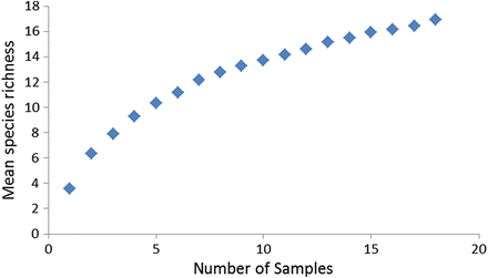
Species accumulation curve
-
5.
How many samples would you need to collect to most accurately and efficiently estimate species richness at this site and sites like it?

5.2.2 Exercise 2. Species Diversity Assessment
Compare the two plant communities below using diversity statistics. Determine which statistics are most helpful, and why.
Community data
Species | Community 1 abundance (percent-cover) | Community 1 abundance (percent-cover) |
A | 30 | 12 |
B | 30 | 12 |
C | 15 | 12 |
D | 15 | 12 |
E | 2 | 12 |
F | 2 | 12 |
G | 2 | 12 |
H | 2 | 12 |
I | 2 | 4 |
Total | 100 | 100 |
-
1.
Simply by inspecting the data, compare the two communities in terms of their species richness and your opinion of their evenness.
-
2.
Calculate Simpson’s Index
Species | Comm1 pi | Comm1 pi 2 | Comm2 pi | Comm2 pi 2 |
A | ||||
B | ||||
C | ||||
D | ||||
E | ||||
F | ||||
G | ||||
H | ||||
I | ||||
Total | D = | D = |
-
3.
Calculate Shannon-Weiner Index
Species | Comm1 pi | Comm1 ln pi | Comm1 pi × ln pi | Comm2 pi | Com21 ln pi | Comm2 pi × ln pi |
A | ||||||
B | ||||||
C | ||||||
D | ||||||
E | ||||||
F | ||||||
G | ||||||
H | ||||||
I | ||||||
Total | H′ = - | H′ = - |
-
4.
Compare the interpretation of the Simpson’s and Shannon-Wiener diversity indices. (A) Which seems to be more effective at distinguishing between the two communities and why? (B) If you were trying to communicate your results to a lay audience, which statistic is easier to interpret and why?
-
5.
Inspect the effective number of species derived from the Simpson’s and Shannon-Wiener indices for the two communities. (A) Do the results from the two communities make sense to you? Why or why not? (B) Is there a difference between the Simpson’s and Shannon Wiener effective number of species? Why do you think this is?
-
6.
Calculate Pielou’s evenness from the Shannon-Wiener index. (Recall that J = H′/ln(S) where S is the species richness.
Pielou’s J: Comm 1: __________ Comm 2: _________
-
7.
Do the evenness statistics make sense given the initial data? Why or why not?
5.2.3 Exercise 3. Calculating an FQAI
Using either data that you collected yourself, or the data provided below, calculate the floristic quality index and mean C of C for the site. If using the provided data set, refer to the University of Wisconsin – Stevens Point herbarium http://wisplants.uwsp.edu/namesearch.html for the coefficient of conservatism (the wetland site is located in Wisconsin). After entering the species name, select the “more information” link for the species C of C.
Provided data set:
Species | Mean abundance (percent-cover) |
Agrostis gigantea | 15 |
Carex atherodes | 42 |
Carex lacustris | 13 |
Carex utriculata | 8 |
Eupatorium perfoliatum | 21 |
Phalaris arundinacea | 52 |
Typha latifolia | 10 |
Calculation table (use your own or provided data set). A typical FQAI does not include abundance data, but only species presence. However, you may have abundance data that you may want to use to weight your findings.
Species | Coefficient of conservatism | Mean abundance | Relative abundance | Weighted C of C (CC′i) |
Sum | A | B | 1.00 | D |
-
\( \mathrm{ A}=\sum\nolimits_i^S {C{C_i}} \)
-
\( \mathrm{ B}=\sum\nolimits_i^S {{x_i}} \) where xi is the mean abundance of species i
-
Relative abundance of species i = \( {{x^{\prime}}_i}={{{{x_i}}} \left/ {\mathrm{ B}} \right.} \)
-
Weighted C of C for species i = \( C{{C^{\prime}}_i}={{x^{\prime}}_i}\times C{C_i} \)
-
D (Weighted C of C of site) = \( \sum\nolimits_i^S {C{{{C^{\prime}}}_i}} \)
-
1.
FQAI = ___________________
-
2.
Mean C of C = ___________________
-
3.
Weighted C of C of site = _________________
-
4.
What does the FQAI tell you about the quality of the wetland site?
-
5.
Do the mean C of C or the weighted C of C provide similar or different interpretations to the FQAI? How are they similar or different?
5.2.4 Exercise 4. Interpreting Multivariate Data
The following figures are output from a multivariate data analysis of 25 Sphagnum species found in 39 different wetlands. Wetlands were clustered into groups based upon their species dissimilarity using hierarchical cluster analysis (Fig. 5.15) and were ordinated within Sphagnum species abundance space using non-metric multidimensional scaling (Fig. 5.16).

Cluster dendrogram of 39 wetlands based upon Sphagnum community dissimilarity. Four groups have been constructed based upon interpretability

NMS ordination of wetlands (labeled P or F) within Sphagnum species space. Wetlands were classified into four groups, named after group indicator species. Centroids of species abundance are labeled by crosses, with the three-letter species abbreviation (e.g., cap= S. capillifolium). Lines are vectors of correlation with environmental variables; longer lines indicate stronger correlation. Micro = microtopographic score, age = time since most recent beaver inhabitation, avegwpH and aveswpH are groundwater and surface water pH, respectively, and avegwspc is mean groundwater specific conductivity
-
1.
Draw a line on the cluster dendrogram where the group cut-off occurs. What percent of information is remaining at this point?
-
2.
If you were to divide the black circle group into four sub-groups, which wetlands would be included in each group?
-
3.
Which wetland group is the least tightly clustered in this ordination diagram?
-
4.
The red/gray lines are correlations of axes with environmental data collected in each wetland. Which wetland group contains the oldest wetlands? Which wetland group contains wetlands with the highest average groundwater specific conductivity?
-
5.
Which group of wetlands is closest to the centroid for S. inundatum on the ordination diagram?
-
6.
What species (three letter abbreviation) is most negatively correlated with Axis 3? Which species is most positively correlated with Axis 3?
-
7.
Which wetland sites (numbers) most likely have the most S. flavicomans?
5.2.5 Exercise 5. Indicator Species
The table below contains data about the distribution of two species in degraded and non-degraded wetlands. Given these data, which species would be a better indicator of degradation and why?
Mean abundance in group/Mean abundance overall | % of sites within group in which species occurs | |||
Degraded | Non-degraded | Degraded | Non-degraded | |
Typha angustifolia | 0.92 | 0.08 | 100 | 10 |
Alnus incana | 0.45 | 0.55 | 60 | 80 |
Rights and permissions
Copyright information
© 2013 Springer Science+Business Media Dordrecht
About this chapter
Cite this chapter
Little, A. (2013). Sampling and Analyzing Wetland Vegetation. In: Anderson, J., Davis, C. (eds) Wetland Techniques. Springer, Dordrecht. https://doi.org/10.1007/978-94-007-6860-4_5
Download citation
DOI: https://doi.org/10.1007/978-94-007-6860-4_5
Published:
Publisher Name: Springer, Dordrecht
Print ISBN: 978-94-007-6859-8
Online ISBN: 978-94-007-6860-4
eBook Packages: Biomedical and Life SciencesBiomedical and Life Sciences (R0)