Abstract
Choice logics constitute a family of propositional logics and are used for the representation of preferences, with especially qualitative choice logic (QCL) being an established formalism with numerous applications in artificial intelligence. While computational properties and applications of choice logics have been studied in the literature, only few results are known about the proof-theoretic aspects of their use. We propose a sound and complete sequent calculus for preferred model entailment in QCL, where a formula F is entailed by a QCL-theory T if F is true in all preferred models of T. The calculus is based on labeled sequent and refutation calculi, and can be easily adapted for different purposes. For instance, using the calculus as a cornerstone, calculi for other choice logics such as conjunctive choice logic (CCL) can be obtained in a straightforward way.
You have full access to this open access chapter, Download conference paper PDF
1 Introduction
Choice logics are propositional logics for the representation of alternative options for problem solutions [4]. These logics add new connectives to classical propositional logic that allow for the formalization of ranked options. A prominent example is qualitative choice logic (QCL for short) [7], which adds the connective ordered disjunction  to classical propositional logic. Intuitively,
  means that if possible A, but if A is not possible than at least B. The semantics of a choice logic induce a preference ordering over the models of a formula.
As choice logics are well suited for preference handling, they have a multitude of applications in AI such as logic programming [8], alert correlation [3], or database querying [13]. But while computational properties and applications of choice logics have been studied in the literature, only few results are known about the proof-theoretic aspects of their use. In particular, there is no proof system capable of deriving valid sentences containing choice operators. In this paper we propose a sound and complete calculus for preferred model entailment in QCL that can easily be generalized to other choice logics.
Entailment in choice logics is non-monotonic: conclusions that have been drawn might not be derivable in light of new information. It is therefore not surprising that choice logics are related to other non-monotonic formalisms. For instance, it is known [7] that QCL can capture propositional circumscription and that, if additional symbols in the language are admitted, circumscription can be used to generate models corresponding to the inclusion-preferred QCL models up to the additional atoms. We do not intend to use this translation of our choice logic formulas (or sequents) in order to employ an existing calculus for circumscription, for instance [5].
Instead, we define calculi in sequent format directly for choice logics, which are different from existing non-monotonic logics in the way non-monotonicity is introduced. Specifically, the non-standard part of our logics is a new logical connective which is fully embedded in the logical language. For this reason, calculi for choice logics also differ from most other calculi for non-monotonic logics: our calculi do not use non-standard inference rules as in default logic, modal operators expressing consistency or belief as in autoepistemic logic, or predicates whose extensions are minimized as in circumscription. However, one method that can also be applied to choice logics is the use of a refutation calculus (also known as rejection or antisequent calculus) axiomatising invalid formulas, i.e., non-theorems. Refutation calculi for non-monotonic logics were used in [5]. Specifically, by combining a refutation calculus with an appropriate sequent calculus, elegant proof systems for the central non-monotonic formalisms of default logic [16], autoepistemic logic [15], and circumscription [14] were obtained. However, to apply this idea to choice logics, we have to take another facet of their semantics into account.
With choice logics, we are working in a setting similar to many-valued logics. Interpretations ascribe a natural number called satisfaction degree to choice logic formulas. Preferred models of a formula are then those models with the least degree. There are several kinds of sequent calculus systems for many-valued logics, where the representation as a hypersequent calculus [1, 10] plays a prominent role. However, there are crucial differences between choice logics and many-valued logics in the usual sense. Firstly, choice logic interpretations are classical, i.e., they set propositional variables to either true or false. Secondly, non-classical satisfaction degrees only arise when choice connectives, e.g. ordered disjunction in QCL, occur in a formula. Thirdly, when applying a choice connective \(\circ \) to two formulas A and B, the degree of \(A \circ B\) does not only depend on the degrees of A and B, but also on the maximum degrees that A and B can possibly assume. Therefore, techniques used in proof systems for conventional many-valued logics can not be applied directly to choice logics.
In [11] a sequent calculus based system for reasoning with contrary-to-duty obligations was introduced, where a non-classical connective was defined to capture the notion of reparational obligation, which is in force only when a violation of a norm occurs. This is related to the ordered disjunction in QCL, however, based on the intended use in [11] the system was defined only for the occurrence of the new connective on the right side of the sequent sign. We aim for a proof system for reasoning with choice logic operators, and to deduce formulas from choice logic formulas. Thus, we need a calculus with left and right inference rules.
To obtain such a calculus we combine the idea of a refutation calculus with methods developed for multi-valued logics in a novel way. First, we develop a (monotonic) sequent calculus for reasoning about satisfaction degrees using a labeled calculus, a method developed for (finite) many-valued logics [2, 9, 12]. Secondly, we define a labeled refutation calculus for reasoning about invalidity in terms of satisfaction degrees. Finally, we join both calculi to obtain a sequent calculus for the non-monotonic entailment of QCL. To this end, we introduce a new, non-monotonic inference rule that has sequents of the two labeled calculi as premises and formalizes degree minimization.
The rest of this paper is organized as follows. In the next section we present the basic notions of choice logics and introduce the most prominent choice logics QCL and CCL (conjunctive choice logic). In Sect. 3 we develop a labeled sequent calculus for propositional logic extended by the QCL connective  . This calculus is shown to be sound and complete and already can be used to derive interesting sentences containing choice operators. In Sect. 4 we extend the previously defined sequent calculus with an appropriate refutation calculus and non-monotonic reasoning, to capture entailment in QCL. The developed methodology for QCL can be extended to other choice logics as well. In particular we show in Sect. 5 how the calculi can be adapted for CCL.
2 Choice Logics
First, we formally define the notion of choice logics in accordance with the choice logic framework of [4] before giving concrete examples in the form of QCL and CCL. Finally, we define preferred model entailment.
Definition 1
Let \(\mathcal {U}\) denote the alphabet of propositional variables. The set of choice connectives \(\mathcal {C}_{\mathcal {L}}\) of a choice logic \(\mathcal {L}\) is a finite set of symbols such that \(\mathcal {C}_{\mathcal {L}} \cap \{\lnot , \wedge , \vee \} = \emptyset \). The set \(\mathcal {F}_{\mathcal {L}}\) of formulas of \(\mathcal {L}\) is defined inductively as follows: (i) \(a \in \mathcal {F}_{\mathcal {L}}\) for all \(a \in \mathcal {U}\); (ii) if \(F \in \mathcal {F}_{\mathcal {L}}\), then \((\lnot F) \in \mathcal {F}_{\mathcal {L}}\); (iii) if \(F, G \in \mathcal {F}_{\mathcal {L}}\), then \((F \circ G) \in \mathcal {F}_{\mathcal {L}}\) for \(\circ \in (\{\wedge , \vee \} \cup \mathcal {C}_{\mathcal {L}})\).
For example,  and
and  . Formulas that do not contain a choice connective are referred to as classical formulas.
The semantics of a choice logic is given by two functions, satisfaction degree and optionality. The satisfaction degree of a formula given an interpretation is either a natural number or \(\infty \). The lower this degree, the more preferable the interpretation. The optionality of a formula describes the maximum finite satisfaction degree that this formula can be ascribed, and is used to penalize non-satisfaction.
Definition 2
The optionality of a choice connective \(\circ \in \mathcal {C}_{\mathcal {L}}\) in a choice logic \(\mathcal {L}\) is given by a function \( opt _{{\mathcal {L}}}^{\circ } :\mathbb {N}^2 \rightarrow \mathbb {N}\) such that \( opt _{{\mathcal {L}}}^{\circ }(k,\ell ) \le (k+1)\cdot (\ell +1)\) for all \(k,\ell \in \mathbb {N}\). The optionality of an \(\mathcal {L}\)-formula is given via \( opt _{\mathcal {L}} :\mathcal {F}_{\mathcal {L}} \rightarrow \mathbb {N}\) with (i) \( opt _{\mathcal {L}}(a) = 1\) for every \(a \in \mathcal {U}\); (ii) \( opt _{\mathcal {L}}(\lnot F) = 1\); (iii) \( opt _{\mathcal {L}}(F \wedge G) = opt _{\mathcal {L}}(F \vee G) = max ( opt _{\mathcal {L}}(F), opt _{\mathcal {L}}(G))\); (iv) \( opt _{\mathcal {L}}(F \circ G) = opt _{{\mathcal {L}}}^{\circ }( opt _{\mathcal {L}}(F), opt _{\mathcal {L}}(G))\) for every choice connective \(\circ \in \mathcal {C}_{\mathcal {L}}\).
The optionality of a classical formula is always 1. Note that, for any choice connective \(\circ \), the optionality of \(F \circ G\) is bounded such that \( opt _{\mathcal {L}}(F \circ G) \le ( opt _{\mathcal {L}}(F)+1) \cdot ( opt _{\mathcal {L}}(G)+1)\). In the following, we write \(\overline{\mathbb {N}}\) for \((\mathbb {N}\cup \{\infty \})\).
Definition 3
The satisfaction degree of a choice connective \(\circ \in \mathcal {C}_{\mathcal {L}}\) in a choice logic \(\mathcal {L}\) is given by a function \({ deg _{{\mathcal {L}}}^{\circ } :\mathbb {N}^{2} \times {\overline{\mathbb {N}}}^{2} \rightarrow \overline{\mathbb {N}}}\) such that \( deg _{{\mathcal {L}}}^{\circ }(k,\ell ,m,n) \le opt _{{\mathcal {L}}}^{\circ }(k,\ell )\) or \( deg _{{\mathcal {L}}}^{\circ }(k,\ell ,m,n) = \infty \) for all \(k,\ell \in \mathbb {N}\) and all \(m,n \in \overline{\mathbb {N}}\). The satisfaction degree of an \(\mathcal {L}\)-formula under an interpretation \(\mathcal {I}\subseteq \mathcal {U}\) is given via the function \( deg _{\mathcal {L}} :2^{\mathcal {U}} \times \mathcal {F}_{\mathcal {L}} \rightarrow \overline{\mathbb {N}}\) with
-
1.
\( deg _{\mathcal {L}}(\mathcal {I},a) = 1 \text { if } a \in \mathcal {I}, deg _{\mathcal {L}}(\mathcal {I},a) = \infty \text { otherwise}\) for every \(a \in \mathcal {U}\);
-
2.
\( deg _{\mathcal {L}}(\mathcal {I},\lnot F) = 1 \text { if } deg _{\mathcal {L}}(\mathcal {I},F) = \infty , deg _{\mathcal {L}}(\mathcal {I},\lnot F) = \infty \text { otherwise}\);
-
3.
\( deg _{\mathcal {L}}(\mathcal {I},F \wedge G) = max ( deg _{\mathcal {L}}(\mathcal {I},F), deg _{\mathcal {L}}(\mathcal {I},G))\);
-
4.
\( deg _{\mathcal {L}}(\mathcal {I},F \vee G) = min ( deg _{\mathcal {L}}(\mathcal {I},F), deg _{\mathcal {L}}(\mathcal {I},G))\);
-
5.
\( deg _{\mathcal {L}}(\mathcal {I},F \circ G) = deg _{{\mathcal {L}}}^{\circ }( opt _{\mathcal {L}}(F), opt _{\mathcal {L}}(G), deg _{\mathcal {L}}(\mathcal {I},F), deg _{\mathcal {L}}(\mathcal {I},G))\), \(\circ \in \mathcal {C}_{\mathcal {L}}\).
We also write \(\mathcal {I}\models ^{\mathcal {L}}_{m} F\) for \( deg _{\mathcal {L}}(\mathcal {I},F) = m\). If \(m < \infty \), we say that \(\mathcal {I}\) satisfies F (to a finite degree), and if \(m = \infty \), then \(\mathcal {I}\) does not satisfy F. If F is a classical formula, then \({\mathcal {I}\models ^{\mathcal {L}}_{1} F \iff \mathcal {I}\models F}\) and \({\mathcal {I}\models ^{\mathcal {L}}_{\infty } F \iff \mathcal {I}\not \models F}\). The symbols \(\top \) and \(\bot \) are shorthand for the formulas \((a \vee \lnot a)\) and \((a \wedge \lnot a)\), where a can be any variable. We have \( opt _{\mathcal {L}}(\top ) = opt _{\mathcal {L}}(\bot ) = 1\), \( deg _{\mathcal {L}}(\mathcal {I},\top ) = 1\) and \( deg _{\mathcal {L}}(\mathcal {I},\bot ) = \infty \) for any interpretation \(\mathcal {I}\) in every choice logic.
Models and preferred models of formulas are defined in the following way:
Definition 4
Let \(\mathcal {L}\) be a choice logic, \(\mathcal {I}\) an interpretation, and F an \(\mathcal {L}\)-formula. \(\mathcal {I}\) is a model of F, written as \(\mathcal {I}\in Mod _{\mathcal {L}}({F})\), if \( deg _{\mathcal {L}}(\mathcal {I},F) < \infty \). \(\mathcal {I}\) is a preferred model of F, written as \(\mathcal {I}\in Prf _{\mathcal {L}}({F})\), if \(\mathcal {I}\in Mod _{\mathcal {L}}({F})\) and \( deg _{\mathcal {L}}(\mathcal {I},F) \le deg _{\mathcal {L}}(\mathcal {J},F)\) for all other interpretations \(\mathcal {J}\).
Moreover, we define the notion of classical counterparts for choice connectives.
Definition 5
Let \(\mathcal {L}\) be a choice logic. The classical counterpart of a choice connective \(\circ \in \mathcal {C}_{\mathcal {L}}\) is the classical binary connective \(\circledast \) such that, for all atoms a and b, \( deg _{\mathcal {L}}(\mathcal {I},a \circ b) < \infty \iff \mathcal {I}\models a \circledast b\). The classical counterpart of an \(\mathcal {L}\)-formula F is denoted as \( cp (F)\) and is obtained by replacing all occurrences of choice connectives in F by their classical counterparts.
A natural property of known choice logics is that choice connectives can be replaced by their classical counterpart without affecting satisfiability, meaning that \( deg _{\mathcal {L}}(\mathcal {I},F) < \infty \iff \mathcal {I}\models cp (F)\) holds for all \(\mathcal {L}\)-formulas F.
So far we introduced choice logics in a quite abstract way. We now introduce two particular instantiations, namely QCL, the first and most prominent choice logic in the literature, and CCL, which introduces a connective  called ordered conjunction in place of QCL’s ordered disjunction.
Definition 6
\(\text {QCL}\) is the choice logic such that  , and, if \(k = opt _{\text {QCL}}(F)\), \(\ell = opt _{\text {QCL}}(G)\), \(m = deg _{\text {QCL}}(\mathcal {I},F)\), and \(n = deg _{\text {QCL}}(\mathcal {I},G)\), then

In the above definition, we can see how optionality is used to penalize non-satisfaction: given a \(\text {QCL}\)-formula  and an interpretation \(\mathcal {I}\), if \(\mathcal {I}\) satisfies F (to some finite degree), then
  ; if \(\mathcal {I}\) does not satisfy F, then
  . Since \( deg _{\text {QCL}}(\mathcal {I},F) \le opt _{\text {QCL}}(F)\), interpretations that satisfy F result in a lower degree, i.e., are more preferable, compared to interpretations that do not satisfy F. Let us take a look at a concrete example:
Example 1
Consider the \(\text {QCL}\)-formula  . Note that the classical counterpart of
  is \(\vee \), i.e., \( cp (F) = (a \vee c) \wedge (b \vee c)\). Thus, \(\{c\},\{a,b\},\{a,c\},\{b,c\},\{a,b,c\} \in Mod _{\text {QCL}}({F})\). Of these models, \(\{a,b\}\) and \(\{a,b,c\}\) satisfy F to a degree of 1 while \(\{c\}\), \(\{a,c\}\), and \(\{b,c\}\) satisfy F to a degree of 2. Therefore, \(\{a,b\},\{a,b,c\} \in Prf _{\text {QCL}}({F})\).
Next, we define \(\text {CCL}\). Note that we follow the revised definition of \(\text {CCL}\) [4], which differs from the initial specificationFootnote 1. Intuitively, given a \(\text {CCL}\)-formula  it is best to satisfy both F and G, but also acceptable to satisfy only F.
Definition 7
\(\text {CCL}\) is the choice logic such that  , and, if \(k = opt _{\text {CCL}}(F)\), \(\ell = opt _{\text {CCL}}(G)\), \(m = deg _{\text {CCL}}(\mathcal {I},F)\), and \(n = deg _{\text {CCL}}(\mathcal {I},G)\), then

Example 2
Consider the \(\text {CCL}\)-formula  . Note that the classical counterpart of
  is the first projection, i.e., \( cp (G) = a \wedge b\). Thus, \(\{a,b\},\{a,b,c\} \in Mod _{\text {CCL}}({G})\). Of these models, \(\{a,b,c\}\) satisfies G to a degree of 1 while \(\{a,b\}\) satisfies G to a degree of 2. Therefore, \(\{a,b,c\} \in Prf _{\text {CCL}}({G})\).
If \(\mathcal {L}\) is a choice logic, then a set of \(\mathcal {L}\)-formulas is called an \(\mathcal {L}\)-theory. An \(\mathcal {L}\)-theory T entails a classical formula F, written as \(T \,\mathrel {\mid \!}\sim F\), if F is true in all preferred models of T. However, we first need to define what the preferred models of a choice logic theory are. There are several approaches for this. In the original QCL paper [7], a lexicographic and an inclusion-based approach were introduced.
Definition 8
Let \(\mathcal {L}\) be a choice logic, \(\mathcal {I}\) an interpretation, and T an \(\mathcal {L}\)-theory. \(\mathcal {I}\in Mod _{\mathcal {L}}({T})\) if \( deg _{\mathcal {L}}(\mathcal {I},F) < \infty \) for all \(F \in T\). \(\mathcal {I}_\mathcal {L}^k(T)\) denotes the set of formulas in T satisfied to a degree of k by \(\mathcal {I}\), i.e., \(\mathcal {I}_\mathcal {L}^k(T) = \{F \in T\mid deg _{\mathcal {L}}(\mathcal {I}, F) = k\}\).
-
\(\mathcal {I}\) is a lexicographically preferred model of T, written as \(\mathcal {I}\in Prf _{\mathcal {L}}^{ lex }(T)\), if \(\mathcal {I}\in Mod _{\mathcal {L}}({T})\) and if there is no \(\mathcal {J}\in Mod _{\mathcal {L}}({T})\) such that, for some \(k \in \mathbb {N}\) and all \(l < k\), \(|\mathcal {I}_\mathcal {L}^k(T)| < |\mathcal {J}_\mathcal {L}^k(T)|\) and \(|\mathcal {I}_\mathcal {L}^l(T)| = |\mathcal {J}_\mathcal {L}^l(T)|\) holds.
-
\(\mathcal {I}\) is an inclusion-based preferred model of T, written as \(\mathcal {I}\in Prf _{\mathcal {L}}^{ inc }(T)\), if \(\mathcal {I}\in Mod _{\mathcal {L}}({T})\) and if there is no \(\mathcal {J}\in Mod _{\mathcal {L}}({T})\) such that, for some \(k \in \mathbb {N}\) and all \(l < k\), \(\mathcal {I}_\mathcal {L}^k(T) \subset \mathcal {J}_\mathcal {L}^k(T)\) and \(\mathcal {I}_\mathcal {L}^l(T) = \mathcal {J}_\mathcal {L}^l(T)\) holds.
In our calculus for preferred model entailment we focus on the lexicographic approach, but it will become clear how it can be adapted to other preferred model semantics (see Sect. 4). We now formally define preferred model entailment:
Definition 9
Let \(\mathcal {L}\) be a choice logic, T an \(\mathcal {L}\)-theory, S a classical theory, and \(\sigma \in \{ lex , inc \}\). \(T \,\mathrel {\mid \!}\sim _\mathcal {L}^\sigma S\) if for all \(\mathcal {I}\in Prf _{\mathcal {L}}^{\sigma }(T)\) there is \(F \in S\) such that \(\mathcal {I}\models F\).
Example 3
Consider the \(\text {QCL}\)-theory  . Then \(\{c\},\{a,c\},\{b,c\} \in Mod _{\text {QCL}}({T})\). Note that, because of \(\lnot (a \wedge b)\), a model of T can not satisfy both
  and
and  to a degree of 1. Specifically,

Thus, \(\{a,c\},\{b,c\} \in Prf _{\text {QCL}}^{ lex }(T)\) but \(\{c\}\not \in Prf _{\text {QCL}}^{ lex }(T)\). It can be concluded that \(T \,\mathrel {\mid \!}\sim _\text {QCL}^ lex c \wedge (a \vee b)\). However,  and
and  .
.
It is easy to see that preferred model entailment is non-monotonic. For example,  but
but  .
.
3 The Sequent Calculus \(\mathbf {L}[\mathrm {QCL}]\)
As a first step towards a calculus for preferred model entailment, we propose a labeled calculus [2, 12] for reasoning about the satisfaction degrees of QCL formulas in sequent format and prove its soundness and completeness. One advantage of the sequent calculus format is having symmetrical left and right rules for all connectives, in particular for the choice connectives. This is in contrast to the representation of ordered disjunction in the calculus for deontic logic [11], in which only right-hand side rules are considered.
As the calculus will be concerned with satisfaction degrees rather than preferred models, we need to define entailment in terms of satisfaction degrees. To this end, the formulas occurring in the sequents of our calculus are labeled with natural numbers, i.e., they are of the form \((A)_k\), where A is a choice logic formula and \(k \in \mathbb {N}\). \((A)_k\) is satisfied by those interpretations that satisfy A to a degree of k. Instead of labeling formulas with degree \(\infty \) we use the negated formula, i.e., instead of \((A)_\infty \) we use \((\lnot A)_1\). We observe that \((A)_k\) for \( opt _{\mathcal {L}}(A) > k\) can never have a model. We will deal with such formulas by replacing them with \((\bot )_1\). For classical formulas, we may write A for \((A)_1\).
Definition 10
Let \((A_1)_{k_1}, \dots , (A_m)_{k_m}\) and \((B_1)_{l_1}, \dots , (B_n)_{l_n}\) be labeled \(\text {QCL}\)-formulas. \((A_1)_{k_1}, \dots , (A_m)_{k_m} \vdash (B_1)_{l_1}, \dots , (B_n)_{l_n}\) is a labeled \(\text {QCL}\)-sequent. \({\varGamma \vdash \varDelta }\) is valid iff every interpretation that satisfies all labeled formulas in \(\varGamma \) to the degree specified by the label also satisfies at least one labeled formula in \(\varDelta \) to the degree specified by the label.
Note that entailment in terms of satisfaction degrees, as defined above, is montonic. Frequently we will write \((A)_{<k}\) as shorthand for \((A)_1, \dots , (A)_{k-1}\) and \((A)_{>k}\) for \((A)_{k+1}, \dots , (A)_{ opt _{\text {QCL}}(A)}, (\lnot A)_1\). Moreover, \(\langle \varGamma , (A)_i \vdash \varDelta \rangle _{i<k}\) denotes the sequence of sequents
Analogously, \(\langle \varGamma , (A)_i \vdash \varDelta \rangle _{i>k}\) stands for the sequence of sequents \(\varGamma , (A)_{k+1} \vdash \varDelta \) \(\dots \) \(\varGamma , (A)_{ opt _{\text {QCL}}(A)} \vdash \varDelta \quad \varGamma , (\lnot A)_{1} \vdash \varDelta \).
We define the sequent calculus \(\mathbf {L}[\mathrm {QCL}]\) over labeled sequents below. In addition to introducing inference rules for  we have to modify the inference rules for conjunction and disjunction of propositional \(\mathbf {LK}\). The idea behind the \(\vee \)-left rule is that a model M of \((A)_k\) is only a model of \((A\vee B)_k\) if there is no \(l <k\) s.t. M is a model of \((B)_l\). Therefore, every model of \((A \vee B)_k\) is a model of \(\varDelta \) iff
-
every model of \((A)_k\) is a model of \(\varDelta \) or of some \((B)_l\) with \(l < k\),
-
every model of \((B)_k\) is a model of \(\varDelta \) or of some \((A)_l\) with \(l < k\).
Essentially the same idea works for \(\wedge \)-left but with \(l > k\). For the \(\vee \)-right rule, in order for every model of \(\varGamma \) to be a model of \((A \vee B)_k\), every model of \(\varGamma \) must either be a model of \((A)_k\) or of \((B)_k\) and no model of \(\varGamma \) can be a model of \((A)_l\) for \(l <k\), i.e., \(\varGamma , (A)_l \vdash \bot \). Similarly for \(\wedge \)-right.
Definition 11
(\(\mathbf {L}[\mathrm {QCL}]\)). The axioms of \(\mathbf {L}[\mathrm {QCL}]\) are of the form \((p)_1 \vdash (p)_1\) for propositional variables p. The inference rules are given below. For the structural and logical rules, whenever a labeled formula \((F)_k\) appears in the conclusion of an inference rule it holds that \(k \le opt _{\mathcal {L}}(F)\).
The structural rules are:

The logical rules are:

The rules for ordered disjunction, with \(k \le opt _{\mathcal {L}}(A)\) and \(l \le opt _{\mathcal {L}}(B)\), are:

The degree overflow rulesFootnote 2, with \(k \in \mathbb {N}\), are:

Observe that the modified \(\wedge \) and \(\vee \) inference rules correspond to the \(\wedge \) and \(\vee \) inference rules of propositional \(\mathbf {LK}\) in case we are dealing only with classical formulas. Our \(\wedge \)-left rule splits the proof-tree unnecessarily for classical theories, and the \(\wedge \)-right rule adds an unnecessary third condition \(\varGamma \vdash A,B,\varDelta \). These additional conditions are necessary when dealing with non-classical formulas.
The intuition behind the degree overflow rules is that we sometimes need to fix invalid sequences, i.e., sequences in which a formula F is assigned a label k with \( opt _{\text {QCL}}(F)< k < \infty \).
Example 4
The following is an \(\mathbf {L}[\mathrm {QCL}]\)-proof of a valid sequent.Footnote 3

Example 5
The following proof shows how the \(\wedge r\)-rule can introduce more than three premises. Note that we make use of the \( do l\)-rule in the leftmost branch.

We now show soundness and completeness of \(\mathbf {L}[\mathrm {QCL}]\).
Proposition 1
\(\mathbf {L}[\mathrm {QCL}]\) is sound.
Proof
We show for all rules that they are sound.
-
For (ax) and the structural rules this is clearly the case.
-
\((\lnot r)\) and \((\lnot l)\): follows from the fact that \( deg _{\text {QCL}}(\mathcal {I},F) < \infty \iff \mathcal {I}\models cp (F)\) for all \(\text {QCL}\)-formulas F.
-
\((\vee l)\): Assume that the conclusion of the rule is not valid, i.e., there is a model M of \(\varGamma \) and \((A \vee B)_k\) that is not a model of \(\varDelta \). Then, M satisfies either A or B to degree k and neither to a degree smaller than k. Assume M satisfies A to a degree of k, the other case is symmetric. Then M is a model of \(\varGamma \) and \((A)_k\) but, by assumption, neither of \(\varDelta \) nor of \((B)_j\) for any \(j < k\). Hence at least one of the premises is not valid. Analogously for \((\wedge l)\).
-
\((\vee r)\): Assume there is a model M of \(\varGamma \) that is not a model of \(\varDelta \) or of \((A \vee B)_k\). There are two possible cases why M is not a model of \((A \vee B)_k\): (1) M satisfies neither A nor B to degree k. But then the premise \(\varGamma \vdash (A)_k,(B)_k, \varDelta \) is not valid as M is also not a model of \(\varDelta \) by assumption. (2) M satisfies either A or B to a degree smaller than k. Assume that M satisfies A to degree \(j <k\) (the other case is symmetric). Then the premise \(\varGamma , (A)_j \vdash \varDelta \) is not valid. Indeed, M is a model of \(\varGamma \) and \((A)_j\) but not of \(\varDelta \). Analogously for \((\wedge r)\).
-
 and
and  : follows from the fact that \((A)_k\) has the same models as
  for \(k \le opt _{\mathcal {L}}(A)\).
 -
 : Assume the conclusion of the rule is not valid and let M be the model witnessing this. Then M is a model of
  . By definition, M satisfies B to degree l and is not a model of A. However, then it is also a model of \(\varGamma \), \((B)_l\) and \((\lnot A)_1\), which means that the premise is not valid.
 -
 . Assume that both premises are valid, i.e., every model of \(\varGamma \) is either a model of \(\varDelta \) or of \((\lnot A)_1\) and \((B)_l\) with \(l \le opt _{\mathcal {L}}(B)\). Now, by definition, any model that is not a model of A (and hence a model of \((\lnot A)_1\)) and of \((B)_l\) satisfies
  to degree \( opt _{QCL}(A) +l\). Therefore, every model of \(\varGamma \) is either a model of \(\varDelta \) or of
  , which means that the conclusion of the rule is valid.
 -
\(( do l)\): \(\varGamma , \bot \) has no models, i.e., the premise \(\varGamma , \bot \vdash \varDelta \) is valid. Crucially, the sequent \(\varGamma , (A)_{ opt _{\text {QCL}}(A)+k}\) has no models as well since A cannot be satisfied to a degree m with \( opt _{\mathcal {L}}(A)< m < \infty \). \(( do r)\) is clearly sound. \(\square \)
 and
and  : follows from the fact that
  for
for  : Assume the conclusion of the rule is not valid and let M be the model witnessing this. Then M is a model of
  . By definition, M satisfies B to degree l and is not a model of A. However, then it is also a model of
  . Assume that both premises are valid, i.e., every model of
  to degree
  , which means that the conclusion of the rule is valid.
Proposition 2
\(\mathbf {L}[\mathrm {QCL}]\) is complete.
Proof
We show this by induction over the (aggregated) formula complexity of the non-classical formulas.
-
For the base case, we observed that if all formulas are classical and labeled with 1, then all our rules reduce to the classical sequent calculus, which is known to be complete. Moreover, we observe that \((A)_1\) is equivalent to A. Hence, we can turn labeled atoms into classical atoms.
-
Assume that a sequent of the form \(\varGamma , (A)_{ opt _{\text {QCL}}(A)+k} \vdash \varDelta \) with \(k \in \mathbb {N}\) is valid. Since \(\varGamma , \bot \) has no models, \(\varGamma , \bot \vdash \varDelta \) is valid and, by the induction hypothesis, provable. Thus, \(\varGamma , (A)_{ opt _{\text {QCL}}(A)+k} \vdash \varDelta \) is provable using the \(( do l)\) rule.
-
Assume that a sequent \(\varGamma \vdash (A)_{ opt _{\text {QCL}}(A)+k},\varDelta \) is valid. \((A)_{ opt _{\text {QCL}}(A)+k}\) can not be satisfied, i.e., \(\varGamma \vdash \varDelta \) is valid and, by the induction hypothesis, provable. Therefore, \(\varGamma \vdash (A)_{ opt _{\text {QCL}}(A)+k},\varDelta \) is provable using the \(( do r)\) rule.
-
Assume that a sequent of the form \(\varGamma \vdash (\lnot A)_1, \varDelta \) is valid. Then every model of \(\varGamma \) is either a model of \((\lnot A)_1\) or of \(\varDelta \). In other words, every model of \(\varGamma \) that is not a model of \((\lnot A)_1\) (i.e., is model of \( cp (A)\)) is a model of \(\varDelta \). Therefore, every interpretation that is a model of both \(\varGamma \) and \( cp (A)\) must be a model of \(\varDelta \). It follows that \(\varGamma , cp (A) \vdash \varDelta \) is valid and, by the induction hypothesis, provable. Thus, \(\varGamma \vdash (\lnot A)_1, \varDelta \) is provable using the \((\lnot r)\) rule. Similarly for \(\varGamma , (\lnot A)_1 \vdash \varDelta \).
-
Assume that a sequent of the form \(\varGamma , (A\vee B)_k \vdash \varDelta \) is valid, with \(k \le opt _{\mathcal {L}}(A \vee B)\). We claim that then both \(\varGamma , (A)_k \vdash (B)_{<k}, \varDelta \) and \(\varGamma , (B)_k \vdash (A)_{<k}, \varDelta \) are valid. Assume to the contrary that \(\varGamma , (A)_k \vdash (B)_{<k}, \varDelta \) is not valid (the other case is symmetric). Then, there is a model M of \(\varGamma \) and \((A)_k\) that is neither a model of \((B)_{<k}\) nor of \(\varDelta \). But then M is also a model of \(\varGamma \) and \((A\vee B)_k\), but not of \(\varDelta \), which contradicts the assumption that \(\varGamma , (A\vee B)_k \vdash \varDelta \) is valid. Therefore, both \(\varGamma , (A)_k \vdash (B)_{<k}, \varDelta \) and \(\varGamma , (B)_k \vdash (A)_{<k}, \varDelta \) are valid and, by the induction hypothesis, provable. This means that \(\varGamma , (A\vee B)_k \vdash \varDelta \) is provable by \((\vee l)\). Similarly for a sequent of the form \(\varGamma , (A\wedge B)_k \vdash \varDelta \).
-
Assume that a sequent of the form \(\varGamma \vdash (A\vee B)_k, \varDelta \) is valid, with \(k \le opt _{\mathcal {L}}(A \vee B)\). We claim that then for all \(i < k\) the sequents \(\varGamma , (A)_i \vdash \varDelta \) and \(\varGamma , (B)_i \vdash \varDelta \) and \(\varGamma \vdash (A)_k, (B)_k, \varDelta \) are valid. Assume by contradiction that there is an \(i < k\) s.t. \(\varGamma , (A)_i \vdash \varDelta \) is not valid. Then, there is a model M of \(\varGamma \) and \((A)_i\) that is not a model of \(\varDelta \). However, then M is a model of \(\varGamma \) but neither of \(\varDelta \) nor of \((A \vee B)_k\) (as M satisfies \(A \vee B\) to degree \(i \ne k\)), which contradicts our assumption that \(\varGamma \vdash (A\vee B)_k, \varDelta \) is valid. The case that there is an \(i < k\) s.t. \(\varGamma , (B)_i \vdash \varDelta \) is not valid is symmetric. Finally, we assume that \(\varGamma \vdash (A)_k, (B)_k, \varDelta \) is not valid. Then, there is a model M of \(\varGamma \) that is not a model of \((A)_k\), \((B)_k\) or \(\varDelta \). Then, M is model of \(\varGamma \) but neither of \(\varDelta \) nor of \((A \vee B)_k\), contradicting our assumption. Therefore, all sequents listed above must be valid, and, by the induction hypothesis, \(\varGamma \vdash (A\vee B)_k, \varDelta \) is provable. Similarly for a sequent of the form \(\varGamma \vdash (A\wedge B)_k, \varDelta \).
-
Assume that a sequent of the form
 with \(k \le opt _{\text {QCL}}(A)\) is valid. Then \(\varGamma , (A)_k \vdash \varDelta \) is also valid since
  and \((A)_k\) have the same models if \(k \le opt _{\text {QCL}}(A)\). By the induction hypothesis
  is provable. Analogously for sequents of the form
  .
. -
Assume that a sequent of the form
 is valid, with \(l \le opt _{\mathcal {L}}(B)\). We claim that the sequent \(\varGamma , (B)_l, \lnot A \vdash \varDelta \) is then also valid. Indeed, if M is a model of \(\varGamma \), \((B)_l\) and \(\lnot A\), then it is also a model of \(\varGamma \) and
  . Hence, by assumption, M must be a model of \(\varDelta \). From this, we can conclude as before that
  is provable.
 -
Assume that a sequent of the form
 is valid, with \(l \le opt _{\mathcal {L}}(B)\). We claim that then also the sequents \(\varGamma \vdash \lnot A, \varDelta \) and \(\varGamma \vdash (B)_l, \varDelta \) are valid. Assume by contradiction that the first sequent is not valid. This means that there is a model M of \(\varGamma \) that is not a model of either \(\lnot A\) nor of \(\varDelta \). However, then M is a model of A and therefore satisfies
  to a degree smaller than \( opt _{\text {QCL}}(A)\). This contradicts our assumption that
  is valid. Assume now that the second sequent is not valid, i.e., that there is a model M of \(\varGamma \) that is neither a model of \((B)_l\) nor of \(\varDelta \). Then, M cannot be a model of
  and we again have a contradiction to our assumption. As before, it follows by the induction hypothesis that
  is provable. \(\square \)
 with
with  and
and  is provable. Analogously for sequents of the form
  .
. is valid, with
  . Hence, by assumption, M must be a model of
  is provable.
 is valid, with
  to a degree smaller than
  is valid. Assume now that the second sequent is not valid, i.e., that there is a model M of
  and we again have a contradiction to our assumption. As before, it follows by the induction hypothesis that
  is provable.
 So far we have not introduced a cut rule, and as we have shown our calculus is complete without such a rule. However, it is easy to see that we have cut-admissibility, i.e., \(\mathbf {L}[\mathrm {QCL}]\) can be extended by:

Another aspect of our calculus that should be mentioned is that, although \(\mathbf {L}[\mathrm {QCL}]\) is cut-free, we do not have the subformula property. This is especially obvious when looking at the rules for negation, where we use the classical counterpart \( cp (A)\) of QCL-formulas. For example,  in the conclusion of the \(\lnot \)-left rule becomes
  in the premise.
While we believe that \(\mathbf {L}[\mathrm {QCL}]\) is interesting in its own right, the question of how we can use it to obtain a calculus for preferred model entailment arises. Essentially, we have to add a rule that allows us to go from standard to preferred model inferences. As a first approach we consider theories \(\varGamma \cup \{A\}\) with \(\varGamma \) consisting only of classical formulas and A being a \(\text {QCL}\)-formula. In this simple case, preferred models of \(\varGamma \cup \{A\}\) are those models of \(\varGamma \cup \{A\}\) that satisfy A to the smallest possible degree. One might add the following rule to \(\mathbf {L}[\mathrm {QCL}]\):

Intuitively, the above rule states that, if there are no interpretations that satisfy \(\varGamma \) while also satisfying A to a degree lower than k, and if \(\varDelta \) follows from all models of \(\varGamma ,(A)_k\), then \(\varDelta \) is entailed by the preferred models of \(\varGamma \cup \{A\}\). However, the obtained calculus  derives invalid sequents.
Example 6
The invalid entailment  can be derived via \(\,\mathrel {\mid \!}\sim _{ naive }\).

What is missing is an assertion that \(\varGamma , (A)_k\) is satisfiable. Unfortunately, this can not be formulated in \(\mathbf {L}[\mathrm {QCL}]\). A way of addressing this problem is to define a refutation calculus, as has been done for other non-monotonic logics [5].
4 Calculus for Preferred Model Entailment
We now introduce a calculus for preferred model entailment. However, as argued above, we first need to introduce the refutation calculus \(\mathbf {L}[\mathrm {QCL}]^{-}\). In the literature, a rejection method for first-order logic with equality was first introduced in [17] and proved complete w.r.t. finite model theory. Our refutation calculus is based on a simpler rejection method for propositional logic defined in [5]. Using the refutation calculus, we prove that \((A)_k\) is satisfiable by deriving the antisequent \((A)_k \nvdash \bot \).
Definition 12
A labeled \(\text {QCL}\)-antisequent is denoted by \(\varGamma \nvdash \varDelta \) and it is valid if and only if the corresponding labeled \(\text {QCL}\)-sequent \(\varGamma \vdash \varDelta \) is not valid, i.e., if at least one model that satisfies all formulas in \(\varGamma \) to the degree specified by the label satisfies no formula in \(\varDelta \) to the degree specified by the label.
Below we give a definition of the refutation calculus \(\mathbf {L}[\mathrm {QCL}]^{-}\). Note that most rules coincide with their counterparts in \(\mathbf {L}[\mathrm {QCL}]\). Binary rules are translated into two rules; one inference rule per premise. \((\vee r)\) and \((\wedge l)\) in \(\mathbf {L}[\mathrm {QCL}]\) have an unbounded number of premises, but due to their structure they can be translated into three inference rules. For \((\wedge r)\) we need to introduce two extra rules for the case that either A or B is not satisfied.
Definition 13
(\(\mathbf {L}[\mathrm {QCL}]^{-}\)). The axioms of \(\mathbf {L}[\mathrm {QCL}]^{-}\) are of the form \(\varGamma \nvdash \varDelta \), where \(\varGamma \) and \(\varDelta \) are disjoint sets of atoms and \(\bot \not \in \varGamma \). The inference rules of \(\mathbf {L}[\mathrm {QCL}]^{-}\) are given below. Whenever a labeled formula \((F)_k\) appears in the conclusion of an inference rule it holds that \(k \le opt _{\mathcal {L}}(F)\).
The logical rules are:

where \(i < k\).

where \(i > k\).
The rules for ordered disjunction, with \(k \le opt _{\mathcal {L}}(A)\) and \(l \le opt _{\mathcal {L}}(B)\), are:

The degree overflow rules, with \(k \in \mathbb {N}\), are:

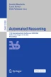
Example 7
The following is related to Example 4 and shows that the sequent  is satisfiable.

Note that the interpretation \(\{a,c\}\) witnesses \((a \vee b), c, \lnot b \nvdash a \wedge b, \bot \).
Proposition 3
\(\mathbf {L}[\mathrm {QCL}]^{-}\) is sound.
Proof
The soundness of the negation rules is straightforward. The soundness of the rules  ,
,  and
and  follows by the same argument as for \(\mathbf {L}[\mathrm {QCL}]\). For the remaining rules, it is easy to check that the same model witnessing the validity of the premise also witnesses the validity of the conclusion. \(\square \)
Proposition 4
\(\mathbf {L}[\mathrm {QCL}]^{-}\) is complete.
Proof
We show completeness by an induction over the (aggregated) formula complexity. Assume \(\varGamma \nvdash \varDelta \) is valid, i.e. \(\varGamma \vdash \varDelta \) is not valid. Now, there must be a rule in \(\mathbf {L}[\mathrm {QCL}]\) for which \(\varGamma \vdash \varDelta \) is the conclusion. By the soundness of \(\mathbf {L}[\mathrm {QCL}]\), this implies that at least one of the premises \(\varGamma ^* \vdash \varDelta ^*\) is not valid. However, then \(\varGamma ^* \nvdash \varDelta ^*\) is valid and, by induction, also provable. Now, by the construction of \(\mathbf {L}[\mathrm {QCL}]^{-}\), there is a rule that allows us to derive \(\varGamma \nvdash \varDelta \) from \(\varGamma ^* \nvdash \varDelta ^*\). \(\square \)
So far no cut-rule has been introduced for \(\mathbf {L}[\mathrm {QCL}]^{-}\), and indeed, a counterpart of the cut rule would not be sound. One possibility is to introduce a contrapositive of cut as described by Bonatti and Olivetti [5]. Again, it is easy to see that this rule is admissible in our calculus:

We are now ready to combine \(\mathbf {L}[\mathrm {QCL}]\) and \(\mathbf {L}[\mathrm {QCL}]^{-}\) by defining an inference rule that allows us to go from labeled sequents to non-monotonic inferences. Again, we first consider the case where \(\varGamma \) is classical and A is a choice logic formula. The preferred model inference rule is:

Intuitively, the premises \(\langle \varGamma , (A)_i \vdash \bot \rangle _{i < k}\) along with \(\varGamma , (A)_k \nvdash \bot \) ensure that models satisfying A to a degree of k are preferred, while the premise \(\varGamma , (A)_k \vdash \varDelta \) ensures that \(\varDelta \) is entailed by those preferred models.
Example 8
The valid entailment  is provable by choosing \(k = 2\):

with \(\varGamma = \lnot (a \wedge b)\) and \(\varDelta = a \wedge c, b\). \(\varphi _3\) is the \(\mathbf {L}[\mathrm {QCL}]\)-proof from Example 4 and \(\varphi _2\) is the \(\mathbf {L}[\mathrm {QCL}]^{-}\)-proof from Example 7. \(\varphi _1\) is not shown explicitly, but it can be verified that the corresponding sequent is provable.
We extend  to the more general case, where more than one non-classical formula may be present, to obtain a calculus for preferred model entailment. An additional rule
  is needed in case a theory is classically unsatisfiable.
Definition 14
(  ). Let \(\le _l\) be the order on vectors in \(\mathbb {N}^k\) defined by
-
\(\mathbf {v} <_l \mathbf {w}\) if there is some \(n \in \mathbb {N}\) such that \(\mathbf {v}\) has more entries of value n and for all \(1 \le m < n\) both vectors have the same number of entries of value m.
-
\(\mathbf {v} =_l \mathbf {w}\) if, for all \(n \in \mathbb {N}\), \(\mathbf {v}\) and \(\mathbf {w}\) have the same number of entries of value n.
 consists of the axioms and rules of \(\mathbf {L}[\mathrm {QCL}]\) and \(\mathbf {L}[\mathrm {QCL}]^{-}\) plus the following rules, where \(\mathbf {v}, \mathbf {w} \in \mathbb {N}^k\), \(\varGamma \) consists of only classical formulas, and every \(A_i\) with \(1 \le i \le k\) is a \(\text {QCL}\)-formula:

We first provide a small example and then show soundness and completeness.
Example 9
Consider the valid entailment  similar to Example 8, but with the information that we require
  and
and  encoded as separate formulas. It is not possible to satisfy all formulas on the left to a degree of 1. Rather, it is optimal to either satisfy
  or, alternatively,
  . We choose \(\mathbf {v} = (1,1,2)\), with \(\mathbf {w} = (1,1,1)\) being the only vector \(\mathbf {w}\) s.t. \(\mathbf {w} < \mathbf {v}\). Thus, we get

with \(\varGamma = \lnot (a \wedge b)\) and \(\varDelta = a \wedge c, b\). It can be verified that indeed all branches are provable, but we do not show this explicitly here.
Proposition 5
 is sound.
Proof
Consider first the \(\,\mathrel {\mid \!}\sim _{ lex }\)-rule and assume that all premises are derivable. By the soundness of \(\mathbf {L}[\mathrm {QCL}]\) and \(\mathbf {L}[\mathrm {QCL}]^{-}\) they are also valid. From the first set of premises \(\langle \varGamma , (A_1)_{w_1}, \dots , (A_k)_{w_k} \vdash \bot \rangle _{\mathbf {w} < \mathbf {v}}\) we can conclude that if there is some model M of \(\varGamma \) that satisfies \(A_i\) to a degree of \(v_i\) for all \(1 \le i \le k\), then \(M \in Prf _{\text {QCL}}^{ lex }(\varGamma \cup \{A_1,\ldots ,A_k\})\). The premise \(\varGamma , (A_1)_{v_1}, \dots , (A_k)_{v_k} \nvdash \bot \) ensures that there is such a model M. By the last set of premises \(\langle \varGamma , (A_1)_{w_1}, \dots , (A_k)_{w_k} \vdash \varDelta \rangle _{\mathbf {w} = \mathbf {v}}\), we can conclude that all models of \(\varGamma \cup \{A_1,\ldots ,A_k\}\) that are equally as preferred as M, i.e., all \(M' \in Prf _{\text {QCL}}^{ lex }(\varGamma \cup \{A_1,\ldots ,A_k\})\), satisfy at least one formula in \(\varDelta \). Therefore, \(\varGamma , A_1, \ldots , A_k \,\mathrel {\mid \!}\sim _\text {QCL}^ lex \varDelta \) is valid.
Now consider the \(\,\mathrel {\mid \!}\sim _{ unsat }\)-rule and assume that \(\varGamma , cp (A_1), \dots , cp (A_k) \vdash \bot \) is derivable and therefore valid. Thus, \(\varGamma \cup \{A_1,\ldots ,A_k\}\) has no models and therefore also no preferred models. Then \(\varGamma , A_1, \ldots , A_k \,\mathrel {\mid \!}\sim _\text {QCL}^ lex \varDelta \) is valid. \(\square \)
Proposition 6
 is complete.
Proof
Assume that \(\varGamma , A_1, \ldots , A_k \,\mathrel {\mid \!}\sim _\text {QCL}^ lex \varDelta \) is valid. If \(\varGamma \cup \{A_1,\ldots ,A_k\}\) is unsatisfiable then \(\varGamma , cp (A_1), \dots , cp (A_k) \vdash \bot \) is valid, i.e., we can apply the \(\,\mathrel {\mid \!}\sim _ unsat \)-rule. Now consider the case that \(\varGamma \cup \{A_1,\ldots ,A_k\}\) is satisfiable and assume that some preferred model M of \(\varGamma \cup \{A_1,\ldots ,A_k\}\) satisfies \(A_i\) to a degree of \(v_i\) for all \(1 \le i \le k\). Then, we claim that all premises of the rule are valid and, by the completeness of \(\mathbf {L}[\mathrm {QCL}]\) and \(\mathbf {L}[\mathrm {QCL}]^{-}\), also derivable.
Assume by contradiction that one of the premises is not valid. First, consider the case that \(\varGamma , (A_1)_{w_1}, \dots , (A_k)_{w_k} \vdash \bot \) is not valid for some \(\mathbf {w} < \mathbf {w}\). Then there is a model \(M'\) of \(\varGamma \) that satisfies \(A_i\) to a degree of \(w_i\) for all \(1 \le i \le k\). However, this contradicts the assumption that M is a preferred model of \(\varGamma \cup \{A_1,\ldots ,A_k\}\).
Next, assume that \(\varGamma , (A_1)_{v_1}, \dots , (A_k)_{v_k} \nvdash \bot \) is not valid. However, M satisfies \(\varGamma , (A_1)_{v_1}, \dots , (A_k)_{v_k}\) and does not satisfy \(\bot \). Contradiction.
Finally, we assume that \(\varGamma , (A_1)_{w_1}, \dots , (A_k)_{w_k} \vdash \varDelta \) is not valid for some \(\mathbf {w} = \mathbf {v}\). Then, there is a model \(M'\) of \(\varGamma \) that satisfies \(A_i\) to a degree of \(w_i\) for all \(1 \le i \le k\) but does not satisfy any formula in \(\varDelta \). But \(M'\) is a preferred model of \(\varGamma \cup \{A_1,\ldots ,A_k\}\), which contradicts \(\varGamma , A_1, \ldots , A_k \,\mathrel {\mid \!}\sim _\text {QCL}^ lex \varDelta \) being valid. \(\square \)
In this paper, we focused on the lexicographic semantics for preferred models of choice logic theories. However, rules for other semantics, e.g. a rule \(\,\mathrel {\mid \!}\sim _{ inc }\) for the inclusion based approach (cf. Definition 8), can be obtained by simply adapting the way in which vectors over \(\mathbb {N}^k\) are compared (cf. Definition 14).
5 Beyond QCL
QCL was the first choice logic to be described [7], and applications concerned with QCL and ordered disjunction have been discussed in the literature [3, 8, 13]. For this reason, the main focus in this paper lies with QCL. However, as we have seen in Sect. 2, CCL and its ordered conjunction show that interesting logics similar to QCL exist. We will now demonstrate that \(\mathbf {L}[\mathrm {QCL}]\) can easily be adapted for other choice logics. In particular, we introduce \(\mathbf {L}[\mathrm {CCL}]\) in which the rules of \(\mathbf {L}[\mathrm {QCL}]\) for the classical connectives can be retained. All that is needed is to replace the  -rules by appropriate rules for the choice connective
  of \(\text {CCL}\).
Definition 15
(\(\mathbf {L}[\mathrm {CCL}]\)). \(\mathbf {L}[\mathrm {CCL}]\) is \(\mathbf {L}[\mathrm {QCL}]\), except that the  -rules are replaced by the following
  -rules:

where \(k \le opt _{\text {CCL}}(B)\), \(l \le opt _{\text {CCL}}(A)\), and \(1 < m \le opt _{\text {CCL}}(A)\).
Note that, given  with \(1 < m \le opt _{\text {CCL}}(A)\), we need to guess whether
  or
or  has to be applied. We do not define \(\mathbf {L}[\mathrm {CCL}]^{-}\) here, but the necessary rules for
  can be inferred from the
  -rules of \(\mathbf {L}[\mathrm {CCL}]\) in a similar way to how \(\mathbf {L}[\mathrm {QCL}]^{-}\) was derived from \(\mathbf {L}[\mathrm {QCL}]\).
Proposition 7
\(\mathbf {L}[\mathrm {CCL}]\) is sound.
Proof
We consider the newly introduced rules.
-
For
 ,
,  , and
, and  this follows directly from the definition of \(\text {CCL}\).
 -
 . Assume both premises are valid, i.e., every model of \(\varGamma \) is a model of \(\varDelta \) or of \((A)_1\) and \((B)_k\) with \(k \le opt _{\mathcal {L}}(B)\). By definition, any model that satisfies \((A)_1\) and \((B)_k\) satisfies
  to degree k. Thus, every model of \(\varGamma \) is a model of \(\varDelta \) or of
  , which means the conclusion of the rule is valid.
 -
 . Assume both premises are valid, i.e., every model of \(\varGamma \) is either a model of \(\varDelta \) or of \((A)_l\) and \((\lnot B)_1\) with \(l \le opt _{\text {CCL}}(A)\). By definition, any model that satisfies \((A)_l\) and does not satisfy B (and hence satisfies \((\lnot B)_1\)) satisfies
  to degree \( opt _{\text {CCL}}(B)+l\).
 -
 . Assume that the premise is valid, i.e., every model of \(\varGamma \) is either a model of \(\varDelta \) or of \((A)_m\) with \(1 < m \le opt _{\text {CCL}}(A)\). By definition, any model that satisfies \((A)_m\), regardless of what degree this model ascribes to B, satisfies
  to degree \( opt _{\text {CCL}}(B)+m\). \(\square \)
 ,
,  , and
, and  this follows directly from the definition of
  . Assume both premises are valid, i.e., every model of
  to degree k. Thus, every model of
  , which means the conclusion of the rule is valid.
 . Assume both premises are valid, i.e., every model of
  to degree
  . Assume that the premise is valid, i.e., every model of
  to degree
 Proposition 8
\(\mathbf {L}[\mathrm {CCL}]\) is complete.
Proof
We adapt the induction of the proof of Proposition 2:
-
Assume that a sequent of the form
 is valid, with \(k \le opt _{\mathcal {L}}(B)\). All models that satisfy
  must satisfy A to a degree of 1 and B to a degree of k. Thus, \(\varGamma , (A)_1, (B)_k \vdash \varDelta \) is valid, and, by the induction hypothesis,
  is provable. Similarly for the cases
  with \(l \le opt _{\text {CCL}}(A)\), and
  with \(1 < m \le opt _{\text {CCL}}(A)\).
 -
Assume that a sequent of the form
 is valid, with \(k \le opt _{\mathcal {L}}(B)\). We claim that then \(\varGamma \vdash (A)_1, \varDelta \) and \(\varGamma \vdash (B)_k, \varDelta \) are valid. Assume, for the sake of a contradiction, that the first sequent is not valid. This means that there is a model M of \(\varGamma \) that is neither a model of \((A)_1\) nor of \(\varDelta \). However, then M satisfies
  to a degree higher than \( opt _{\text {CCL}}(B)\). This contradicts the assumption that
  is valid. Assume now that the second sequent is not valid, i.e., that there is a model M of \(\varGamma \) that is neither a model of \((B)_k\) nor of \(\varDelta \). Then M cannot be a model of
  , contradicting the assumption. As before, it follows by the induction hypothesis that
  is provable. Similarly for the cases
  with \(l \le opt _{\text {CCL}}(A)\), and
  with \(1 < m \le opt _{\text {CCL}}(A)\). \(\square \)
 is valid, with
  must satisfy A to a degree of 1 and B to a degree of k. Thus,
  is provable. Similarly for the cases
  with
with  with
with  is valid, with
  to a degree higher than
  is valid. Assume now that the second sequent is not valid, i.e., that there is a model M of
  , contradicting the assumption. As before, it follows by the induction hypothesis that
  is provable. Similarly for the cases
  with
with  with
with We are confident that our methods can be adapted not only for QCL and CCL, but for numerous other instantiations of the choice logic framework defined in Sect. 2. We mention here lexicographic choice logic (LCL) [4], in which  expresses that it is best to satisfy A and B, second best to satisfy only A, third best to satisfy only B, and unacceptable to satisfy neither.
Moreover, note that the inference rules \(\,\mathrel {\mid \!}\sim _{ lex }\) and \(\,\mathrel {\mid \!}\sim _{ unsat }\) (cf. Definition 14) do not depend on any specific choice logic. Thus, once labeled calculi are developed for a choice logic, a calculus for preferred model entailment follows immediately.
6 Conclusion
In this paper we introduce a sound and complete sequent calculus for preferred model entailment in QCL. This non-monotonic calculus is built on two calculi: a monotonic labeled sequent calculus and a corresponding refutation calculus.
Our systems are modular and can easily be adapted: on the one hand, calculi for choice logics other than QCL can be obtained by introducing suitable rules for the choice connectives of the new logic, as exemplified with our calculus for CCL; on the other hand, a non-monotonic calculus for preferred model semantics other than the lexicographic semantics can be obtained by adapting the inference rule \(\,\mathrel {\mid \!}\sim _{ lex }\) which transitions from preferred model entailment to the labeled calculi.
Our work contributes to the line of research on non-monotonic sequent calculi that make use of refutation systems [5]. Our system is the first proof calculus for choice logics, which have been studied mainly from the viewpoint of their computational properties [4] and their potential applications [3, 8, 13] so far.
Regarding future work, we aim to investigate the proof complexity of our calculi, and how this complexity might depend on which choice logic or preferred model semantics is considered. Also, calculi for other choice logics such as LCL could be explicitly defined, as was done with CCL in Sect. 5.
Notes
- 1.
It seems that, under the initial definition of CCL,
 is always ascribed a degree of 1 or \(\infty \), i.e., non-classical degrees can not be obtained (cf. Definition 8 in [6]).
 - 2.
\( do l\)/\( do r\) stands for degree overflow left/right.
- 3.
Note that, once we reach sequents containing only classical formulas, we do not continue the proof. However, it can be verified that the classical sequents on the left and right branch are provable in this case. Moreover, given a formula \((A)_1\) with a label of 1, the label is often omitted for readability.
 is always ascribed a degree of 1 or
 References
Avron, A.: The method of hypersequents in the proof theory of propositional nonclassical logics. In: Hodges, W., Hyland, M., Steinhorn, C., Truss, J. (eds.) Logic: From Foundations to Applications, pp. 1–32. Oxford Science Publications, Oxford (1996)
Baaz, M., Lahav, O., Zamansky, A.: Finite-valued semantics for canonical labelled calculi. J. Autom. Reason. 51(4), 401–430 (2013)
Benferhat, S., Sedki, K.: Alert correlation based on a logical handling of administrator preferences and knowledge. In: SECRYPT, pp. 50–56. INSTICC Press (2008)
Bernreiter, M., Maly, J., Woltran, S.: Choice logics and their computational properties. In: IJCAI, pp. 1794–1800. ijcai.org (2021)
Bonatti, P.A., Olivetti, N.: Sequent calculi for propositional nonmonotonic logics. ACM Trans. Comput. Log. 3(2), 226–278 (2002)
Boudjelida, A., Benferhat, S.: Conjunctive choice logic. In: ISAIM (2016)
Brewka, G., Benferhat, S., Berre, D.L.: Qualitative choice logic. Artif. Intell. 157(1–2), 203–237 (2004)
Brewka, G., Niemelä, I., Syrjänen, T.: Logic programs with ordered disjunction. Comput. Intell. 20(2), 335–357 (2004)
Carnielli, W.A.: Systematization of finite many-valued logics through the method of tableaux. J. Symb. Log. 52(2), 473–493 (1987)
Geibinger, T., Tompits, H.: Sequent-type calculi for systems of nonmonotonic paraconsistent logics. In: ICLP Technical Communications. EPTCS, vol. 325, pp. 178–191 (2020)
Governatori, G., Rotolo, A.: Logic of violations: a Gentzen system for reasoning with contrary-to-duty obligations. Australas. J. Logic 4, 193–215 (2006)
Kaminski, M., Francez, N.: Calculi for many-valued logics. Log. Univers. 15(2), 193–226 (2021)
Liétard, L., Hadjali, A., Rocacher, D.: Towards a gradual QCL model for database querying. In: Laurent, A., Strauss, O., Bouchon-Meunier, B., Yager, R.R. (eds.) IPMU 2014. CCIS, vol. 444, pp. 130–139. Springer, Cham (2014). https://doi.org/10.1007/978-3-319-08852-5_14
McCarthy, J.: Circumscription - a form of non-monotonic reasoning. Artif. Intell. 13(1–2), 27–39 (1980)
Moore, R.C.: Semantical considerations on nonmonotonic logic. Artif. Intell. 25(1), 75–94 (1985)
Reiter, R.: A logic for default reasoning. Artif. Intell. 13(1–2), 81–132 (1980)
Tiomkin, M.L.: Proving unprovability. In: LICS, pp. 22–26. IEEE Computer Society (1988)
Acknowledgments
We thank the anonymous reviewers for their valuable feedback. This work was funded by the Austrian Science Fund (FWF) under the grants Y698 and J4581.
Author information
Authors and Affiliations
Corresponding author
Editor information
Editors and Affiliations
Rights and permissions
Open Access This chapter is licensed under the terms of the Creative Commons Attribution 4.0 International License (http://creativecommons.org/licenses/by/4.0/), which permits use, sharing, adaptation, distribution and reproduction in any medium or format, as long as you give appropriate credit to the original author(s) and the source, provide a link to the Creative Commons license and indicate if changes were made.
The images or other third party material in this chapter are included in the chapter's Creative Commons license, unless indicated otherwise in a credit line to the material. If material is not included in the chapter's Creative Commons license and your intended use is not permitted by statutory regulation or exceeds the permitted use, you will need to obtain permission directly from the copyright holder.
Copyright information
© 2022 The Author(s)
About this paper

Cite this paper
Bernreiter, M., Lolic, A., Maly, J., Woltran, S. (2022). Sequent Calculi for Choice Logics. In: Blanchette, J., Kovács, L., Pattinson, D. (eds) Automated Reasoning. IJCAR 2022. Lecture Notes in Computer Science(), vol 13385. Springer, Cham. https://doi.org/10.1007/978-3-031-10769-6_20
Download citation
DOI: https://doi.org/10.1007/978-3-031-10769-6_20
Published:
Publisher Name: Springer, Cham
Print ISBN: 978-3-031-10768-9
Online ISBN: 978-3-031-10769-6
eBook Packages: Computer ScienceComputer Science (R0)