
Abstract
Wireless sensor network (WSN) is formed by a large number of cheap sensors, which are communicated by an ad hoc wireless network to collect information of sensed objects of a certain area. The acquired information is useful only when the locations of sensors and objects are known. Therefore, localization is one of the most important technologies of WSN. In this paper, weighted Voronoi diagram-based localization scheme (W-VBLS) is proposed to extend Voronoi diagram-based localization scheme (VBLS). In this scheme, firstly, a node estimates the distances according to the strength of its received signal strength indicator (RSSI) from neighbor beacons and divides three beacons into groups, whose distances are similar. Secondly, by a triangle, formed by the node and two beacons of a group, a weighted bisector can be calculated out. Thirdly, an estimated position of the node with the biggest RSSI value as weight can be calculated out by three bisectors of the same group. Finally, the position of the node is calculated out by the weighted average of all estimated positions. The simulation shows that compared with centroid and VBLS, W-VBLS has higher positioning accuracy and lower computation complexity.
1 Introduction
Wireless sensor network (WSN) is a self-organizing distributed network system including plenty of tiny sensor nodes with the ability to communicate and calculate in a specific monitoring area. In the wireless sensor network, the node position information plays a very important role in monitoring activity. The monitoring information without location message is meaningless. Therefore, the research of wireless sensor network positioning technology is the key technology of WSN [1].
The existing location algorithm is divided into two major categories which are range-based and range-free. APS [2], AHLoS algorithm [3], trilateration algorithm [4], lateration algorithm [5], and alternating combination trilateration (ACT) [6] are typical range-based algorithms. Centroid algorithm [7], DV-hop algorithm [8], APIT algorithm [9], and amorphous algorithm [10] are typical range-free algorithms.
Literature [11] used Voronoi diagrams in wireless sensor node localization. In this algorithm, the midperpendiculars between each beacon node and its neighbor beacon node composed the Voronoi region boundaries. According to the properties of the Voronoi diagrams, we can see that the node to be located is in its nearest beacon node Voronoi region. Therefore, in literature [11], the algorithm weighted all the nodes within this region firstly and obtained all the beacon nodes’ Voronoi regions in order, then added different weight values to the obtained regions, and finally obtained the centroid of the largest weight value region as the estimated coordinate of the node to be located.
However, algorithm [11] using the midperpendicular of the beacon nodes as Voronoi diagram region boundaries could not reflect the relationship between the RSSI signal strength and the distance among the nodes. Therefore, in order to improve localization accuracy and reduce complexity of the algorithm, we improved the localization algorithm based on Voronoi diagrams. In the improved algorithm, we selected two beacon nodes' weighted bisector as the region boundaries, then calculated the two weighted bisector intersection coordinates as estimate coordinates, and finally we regarded the weighted average values of all the estimate coordinates as the final estimate coordinates of the node to be located.
2 Positioning algorithm based on Voronoi
Voronoi diagram (Figure 1) refers to a point set in a given space, P = {P1, P2, P3,⋯P n }, 3 ≤ n < ∞. The plane is divided by the Voronoi diagram as follows:

Voronoi.
In the previous formula, let x be any point in the plane and d(x, P i ) be the Euclidean distance [11] between x and the certain point P i . In wireless sensor networks, because RSSI signal values between nodes are inversely proportional to the square of their distances, then according to this property and the definition of Voronoi diagrams, we can describe WSN node localization as follows.
-
1.
Let P 1, P 2, P 3,⋯,, P n be beacon nodes in wireless sensor network area and S be node to be located.
-
2.
We can suppose beacon nodes P 1, P 2, P 3,⋯, P j communicate with the node S, and the node S receives RSSI signal strength of the beacon node according to size of .
-
3.
According to the properties of the Voronoi diagrams, we can see that the unknown node S is in the Voronoi region of beacon node P 1. We compute P 1’s Voronoi regions and add the weight values to all the nodes within this area.
-
4.
Remove the node P 1, compute the Voronoi region of P 2, and assign node weight value . In this way, eventually, we can obtain all beacon nodes of the Voronoi regions.
-
5.
We can find the region with a maximum weight value and get the gravity coordinate as the calculation coordinate of the unknown node S.
3 Positioning algorithm based on weighted Voronoi
In Voronoi diagram algorithm, the Voronoi region of beacon node P i is made of midperpendiculars of this beacon node and the beacon nodes around it. However, in fact, if the nodes have the same centroid and the greater the intensity of the RSSI signal the node received, the smaller the distance between nodes will be. Therefore, we can appropriately adjust the Voronoi region of this node through the signal value. Thus, we can improve the localization accuracy and reduce computational complexity.
3.1 Algorithm basic ideas
We presume the node to be located S can receive the signal from beacon nodes P1, P2, P3,⋯, P n . When S has the distance of d i , d j (suppose d i > d j ) to any two beacon nodes P i , P j , the node to be located S and P i , P j will form a triangle SP i P j . Let node S be in the line of P i P j ’s weight bisector; we can select this line as the region boundaries of beacon nodes P i and P j . Then, we can select beacons P m , P n and repeat the above method. We will get a more accurate Voronoi region at last.
Because of the assumption d i > d j , we know ∠ SP i P j > ∠ SP j P i in the triangle SP i P j . For calculating the straight line equation L of weight bisector, we need to get the slope k of L and the intersection coordinates P between P i P j and L. With the properties of the straight slope, the slope of L is the opposite to the reciprocal slope of bottom edge P i P j , that is . We use the following three cases to seek the intersection coordinate P(x0, y0):
-
1.
∠ SP i P j is an acute angle (Figure 2).
Figure 2 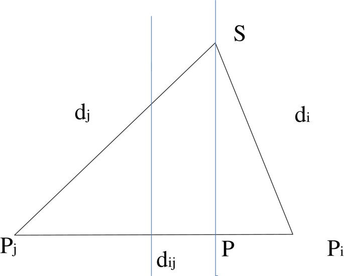
∠ SP i P j is an acute angle.
We calculate the next formula first.
(1)We know s1 and s2 are both greater than zero from the cosine law. Then, we can choose proportionality coefficient as the specific value of and , that, is
(2)Because we have calculated the positions of s1 and s2 and the positions of P1 and P2 have been known, we can get the coordinate P(x0, y0).
(3)Taking k L that we have obtained and P(x0, y0) into the equation y − y0 = k(x − x0), we can receive the equation as follows:
(4) -
2.
∠ SP i P j is a right angle (Figure 3).
Figure 3 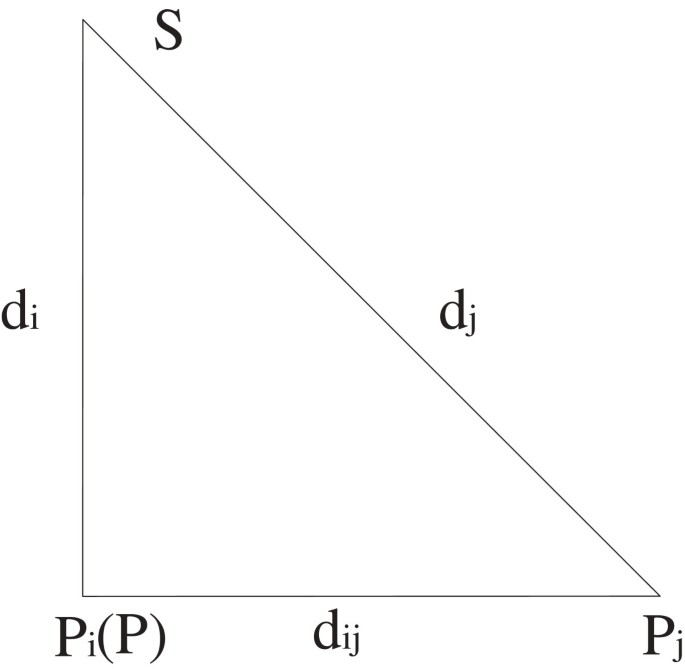
∠ SP i P j is a right angle.
Straight line L is P i S in the triangle, so straight line L’s slope k L is still ; the intersection of L and bottom edge P i P j is P i (x i , y i ). Then, we can get the equation of straight line L:
(5) -
3.
∠ SP i P j is an obtuse angle (Figure 4).
Figure 4 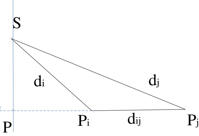
∠ SP i P j is an obtuse angle.
We still calculate
(6)At this time, s1 > 0, s2 < 0; then, the proportionality coefficient is .
In a similar way, we can get the coordinates P(x0, y0).
(7)Then, get the equation of L.
(8)


3.2 Algorithmic process
Localization algorithm based on weighted Voronoi diagrams works as follows:
-
1.
The node to be located S broadcasts around the information Request with requesting location.
-
2.
All beacon nodes that received the Request return the information Reply which contains its own location.
-
3.
After node S receives all the information, we sort the beacon nodes from big to small according to the signal intensity. We assume that the sorted order of beacon nodes is P 1, P 2, P 3,⋯,P k .
-
4.
The bottom edge heights of SP 1 P 2, SP 2 P 3,⋯, SP k − 1 P k form the equations L 1, L 2,⋯,, L k − 1.
-
5.
Next, we can get the intersection Q 1 of L 1 and L 2, Q 2 of L 2 and L 3,⋯, and Q k − 2 of L k − 2 and L k − 1. Then, we attach the RSSI signal values of P 1, P 2,⋯P k − 2 to the nodes Q 1, Q 2,⋯,Q k − 2 as weighted values.
-
6.
Calculate the weighted average coordinates from node Q 1 to node Q k − 2.
4 Experiment and performance analysis of the positioning algorithm
In this section, we make the simulation analysis on performance comparison among the new algorithm, weighted centroid algorithm (W-Centroid) and Voronoi diagram-based localization scheme (VBLS) algorithm by MATLAB 7.0 (The MathWorks, Inc., Natick, MA, USA).
There are 25 beacon nodes distributed randomly in the region of 100 m × 100 m, among which Shadowing model is adopted to realize the communication.
In the previous equation, P r (d0) and d0 represent reference energy and reference distance, respectively. β represents path loss coefficient (general value is 2 ~ 4), and X db is a Gaussian variable that has an average value of zero.
Figure 5 describes the relation between localization accuracy of the three algorithms and communication radius. From Figure 5, we can see that weighted Voronoi diagram-based localization scheme (W-VBLS) algorithm’s relative errors decrease gradually with the increase of communication radius. When the communication radius is greater than 45 m, it is essentially flat with VBLS errors. As communication radius increases, the beacon nodes involved in the localization increases, the unknown node can gain more location information, and localization errors decrease.

The relationship between positioning accuracy and communication radius.
Figure 6 depicts the relation between localization accuracy of the three algorithms and the number of nodes. As can be seen from Figure 6, with the number of beacon nodes increasing, the localization accuracy improves gradually. When beacon node increases to 25, localization accuracy has few changes. In order to locate, the VBLS localization algorithm must have at least four nodes, while the W-VBLS algorithm only needs three beacon nodes. Therefore, in case the beacon nodes are sparse, W-VBLS significantly has higher positioning accuracy than the other two algorithms.

The relationship between positioning accuracy and the number of beacon nodes.
Figure 7 depicts the relationship between the positioning accuracy of the three algorithms and noise. W-Centrold adopts the connectivity among nodes to positioning, while VBLS and W-VBLS positioning base on the size of the RSSI signal. In case the noise increases, W-Centrold positioning algorithm only has small fluctuations, while VBLS and W-VBLS will have fluctuations with noise increasing. When the noise reaches 0.5, positioning errors of the two algorithms are basically the same.

The relationship between accuracy and noise.
5 Conclusion
Based on the research of Voronoi diagram range-free localization algorithm, we propose a Voronoi diagram weighted localization algorithm. The algorithm uses the relationship between the distances among the nodes, and the RSSI signal intensity corrects the Voronoi diagram boundaries. At the same time, it reduces the number of minimum required localization beacon nodes and the complexity of the algorithm and improves the positioning accuracy.
References
Sun L, Li J, Chen Y, Zhu H: Wireless Sensor Network. Bei**g: Tsinghua University Press; 2005:136-154.
Langendoen K, Reijers N: Distributed localization in wireless sensor networks: a quantitative comparison. Comp. Netw. 2003, 42(4):499-518.
Savvides A, Han CC, Strivastava MB: Dynamic fine-grained localization in Ad-hoc networks of sensors. Rome, Italy: Paper presented at the 7th annual international conference on mobile computing and networking; 2001:166-179.
Nicolescu D, Nath B: Ad-hoc positioning systems (APS) using AOA. New York: Paper presented at the 22nd annual joint conference of the IEEE computer and communications; 2003:1734-1743.
Niculescu D, Nath B: Position and orientation in ad hoc networks. Ad Hoc Netw. 2004, 2(2):133-151. 10.1016/S1570-8705(03)00051-9
Yu Y: Sensor Network Positioning Algorithm and Related Technology Research. Chongqing: Chongqing University; 2006.
Bulusu N, Heidemann J, Estrin D: GPS-less low cost outdoor localization for very small devices. IEEE Wirel. Commun. 2000, 7(5):27-34.
Niculescu D, Nath B: DV-based positioning in ad hoc networks. Telecommun. Syst. 2003, 22(1–4):267-280.
He T, Huang C, Blum BM, Stankovic JA, Abdelzaher T: Range-free localization schemes for large scale sensor networks. San Diego, CA, USA: Paper presented at the 9th annual international conference on mobile computing and networking; 2003:81-95.
Nagpal R, Shrobe H, Bachrach J: Organizing a global coordinate system from local information on an ad-hoc sensor network. Palo Alto, CA, USA: Paper presented at the second international conference on information processing in sensor networks; 2003.
Wang J, Huang L, Xu H, Xu B, Li S: Based on Voronoi diagram without ranging wireless sensor network node positioning algorithm. Comput. Res. Dev. 2008, 45(1):119-125.
Acknowledgements
The paper is supported by the National Science Foundation of China (41176082, 61073182), supported by the Program for New Century Excellent Talents in University (NCET-13-0753), Specialized Research Fund for the Doctoral Program of Higher Education (20132304110031), and the Fundamental Research Funds for the Central Universities (HEUCFT1202).
Author information
Authors and Affiliations
Corresponding author
Additional information
Competing interests
The authors declare that they have no competing interests.
Authors’ original submitted files for images
Below are the links to the authors’ original submitted files for images.
Rights and permissions
Open Access This article is distributed under the terms of the Creative Commons Attribution 2.0 International License (https://creativecommons.org/licenses/by/2.0), which permits unrestricted use, distribution, and reproduction in any medium, provided the original work is properly cited.
About this article
Cite this article
Cai, S., Pan, H., Gao, Z. et al. Research of localization algorithm based on weighted Voronoi diagrams for wireless sensor network. J Wireless Com Network 2014, 50 (2014). https://doi.org/10.1186/1687-1499-2014-50
Received:
Accepted:
Published:
DOI: https://doi.org/10.1186/1687-1499-2014-50