
Abstract
The advent of high-resolution electron and scanning probe microscopy imaging has opened the floodgates for acquiring atomically resolved images of bulk materials, 2D materials, and surfaces. This plethora of data contains an immense volume of information on materials structures, structural distortions, and physical functionalities. Harnessing this knowledge regarding local physical phenomena necessitates the development of the mathematical frameworks for extraction of relevant information. However, the analysis of atomically resolved images is often based on the adaptation of concepts from macroscopic physics, notably translational and point group symmetries and symmetry lowering phenomena. Here, we explore the bottom-up definition of structural units and symmetry in atomically resolved data using a Bayesian framework. We demonstrate the need for a Bayesian definition of symmetry using a simple toy model and demonstrate how this definition can be extended to the experimental data using deep learning networks in a Bayesian setting, namely rotationally invariant variational autoencoders.
Introduction
Macroscopic symmetry is one of the central concepts in the modern condensed matter physics and materials science1,2,3,4,5,6. Formalized via point and spatial group theory, symmetry underpins areas such as structural analysis, serves as the basis for the descriptive formalism of quasiparticles and elementary excitations, phase transitions, and mesoscopic order-parameter-based descriptions, especially of crystalline solids. In macroscopic physics, symmetry concepts arrived with the advent of X-ray methods developed by Bragg, and for almost a century remained the primary and natural language of physics. Notably, the rapid propagation of laboratory X-ray diffractometers and large-scale X-ray scattering facilities provided ample experimental data across multiple material classes and serve as a necessary counterpart for theoretical developments. Correspondingly, symmetry-based descriptors have emerged as a foundational element of condensed matter physics and materials science alike.
The natural counterpart of symmetry-based descriptors is the concept of physical building blocks. Thus, crystalline solids can be generally described via a combination of the unit cells with discrete translational lattice symmetries2,3,7. At the same time, systems such as Penrose structures8,9,10,11,12,13 possess well-defined building blocks but undefined translation symmetry. Finally, a broad range of materials lack translational symmetries, with examples ranging from structural glasses and polymers to ferroelectric and magnetic morphotropic systems14,15,16,17,18,19,20,21,22. Remarkably, the amenability of symmetry-based descriptors have led to much deeper insights into the structure and functionalities of materials with translational symmetries compared to (partially) disordered systems23,24,25.
The beginning of the 21st century has seen the emergence of real space imaging methods including scanning probe microscopy (SPM)26,27,28 and especially (scanning) transmission electron microscopy ((S)TEM)29,30,31. Following the introduction of the aberration corrector in the late ‘90s32 and the advent of commercial aberration-corrected microscopes, atomically resolved imaging is now mainstream. Notably, modern STEMs allow atomic columns to be imaged with ~pm-level precision33. This level of structural information allows insight into the chemical and physical functionalities of materials, including chemical reactivity, magnetic, and dielectric properties utilizing structure-property correlations developed by condensed matter physicists from macroscopic scattering data34,35,36,37,38,39,40. Over the last decade, several groups have extended these analyses to derive mesoscopic order parameter fields such as polarization41,42,43,44, strains and chemical strains45, and octahedra tilts46,47,48 directly from STEM and SPM data. Strain measurements have also been done in reciprocal space using nano-diffraction49, ultrafast CBED50, and a combination of 4D-STEM and machine learning51. In several cases, these data can be matched to the mesoscopic Ginzburg-Landau models, providing insight into the generative mesoscopic physics of the material52,53. Recently, a similar approach was proposed and implemented for theory-experiment matching via microscopic degrees of freedom54,55,56.
Yet, despite the wealth of information contained in atomically resolved imaging data, analyses to date were almost invariably based on the mathematical apparatus developed for macroscopic scattering data57,58,59,60,61. However, the nature of microscopic measurements is fundamentally different. For the case of ideal single crystal containing a macroscopic number of structural units, the symmetry of the diffraction pattern represents that of the lattice and the width of the peaks in Fourier space is determined by the intrinsic factors such as angle resolution of the measurement system, rather than disorder in the material. The presence of symmetry breaking distortions, such as the transition from a cubic to tetragonal state, is instantly detectable from peak splitting. For microscopic observations only a small part of the object is visible and the positions of the atoms are known only within an uncertainty interval; this uncertainty can be comparable to the magnitude of the symmetry breaking feature of interest such as tetragonality or polarization. Thus, questions arise: What image size is it justified to define the symmetry from the atomically resolved data? and What level of confidence can be defined? Ideally, such an approach should be applicable not only for structural data, but also for more complex multi-dimensional data sets such as those available in scanning tunneling spectroscopy (STS)62 in scanning tunneling microscopy (STM), force-distance curve imaging63 in atomic force microscopy, or electron energy loss spectroscopy (EELS)64,65 and ptychographic imaging66,67,68 in scanning transmission electron microscopy (STEM).
Here we propose an approach for the analysis of spatially resolved data based on deep learning in a Bayesian setting. This analysis utilizes the synergy of three fundamental concepts; the (postulated) parsimony of the atomic-level descriptors corresponding to stable atomic configurations, the presence of distortions in the idealized descriptors (e.g., due to local strains or other forms of symmetry breaking), and the presence of possible discrete or continuous rotational symmetries. These concepts are implemented in a workflow combining feature selection (atom finding), a rotationally invariant variational autoencoder to determine symmetry invariant building blocks, and a conditional autoencoder to explore intra-class variability via relevant disentangled representations. This approach is demonstrated for 2D imaging data but can also be generalized for more complex multi-dimensional data sets.
Results and discussion
Why local symmetry is Bayesian
Here, we illustrate why the consistent definitions of local symmetry properties necessitates the Bayesian framework. As an elementary, but easy to generalize example, we consider the 1D diatomic chain formed by alternating atoms (1) and (2) with coordinates generated by the rule \(x_i^{(1)} = x_i^{(2)} + a\), \(x_{i + 1}^{(2)} = x_i^{(1)} + b\). The atomic coordinates with some uncertainty stemming from the observational noise, sampling, etc. are experimentally observed and hence, the atomic positions, \(x_j^{exp}\), that are the sum of the ideal positions, \(x_j^{(1,2)}\), and noise, \(\delta\), are available for observation. We assume that the atom types are not observed (e.g. they have similar contrast), i.e., atoms (1) and (2) are indistinguishable. Correspondingly, we aim to answer the question - what number of observations can distinguish the simple chain, a = b, and diatomic chain, \(a \ne b\)? Note that this problem is equivalent to, e.g., distinguishing a square and tetragonal unit cell and can be generalized to more complex cases with the addition of several parameters.
The classical answer to this question is given by frequency-based statistics. Here, an alternative hypothesis (i.e. single vs. double chain) is formed where the point estimates for the average lattice parameters and their dispersions are calculated and the p-test can be used determine the correctness of the hypothesis. However, this approach has several significant limitations: it does not consider any potential prior knowledge of the system, it implicitly relies on the relevant distributions being Gaussian, and it is sensitive to the choice of an ideal system. A detailed analysis of the relevant drawbacks is given by Kruschke69.
An alternative approach to these problems is via the Bayesian framework, based on the concept of prior and posterior probabilities linked as70,71:
where D represents the data obtained during the experiment, \(p\left( {D|\theta _i} \right)\) represents the likelihood that this data can be generated by the model, i, with parameter, \(\theta _i\). The prior, \(p\left( {\theta _i} \right)\), reflects the prior knowledge about the model. The posterior, \(p\left( {\theta _i|D} \right)\), describes the new knowledge (i.e., updated model and model parameters) as a result of the observational data. Finally, \(p\left( D \right)\) is the denominator that defines the total space of possible outcomes.
As an example, a set of diatomic chains is generated with bond lengths derived from two normal distributions, N(µ = 0.5, σ2 = 0.01) and N(µ = 1.5, σ2 = 0.01), where μ is the mean and σ the standard deviation of the distribution. These two sets of bond lengths are treated independently and are referred to as odd and even bond lengths, respectively. The likely distributions for this case are also assumed to be normal distributions, N(µ = µ1, σ = σ1) and N(µ = µ2, σ = σ2). A total of four parameters, µ1 and σ1for the odd bond lengths and µ2 and σ2 for the even bond lengths, exhaustively determine the parameter space. We refer to this analysis as case-1.
The key element of Bayesian inference is the concept of prior, summarizing the known information on the system70,71,72. In experiments, the priors are typically formed semi-quantitatively based on general physical knowledge of the material (e.g., SrTiO3 is known to be cubic with lattice parameter 3.1 Å). For this model example, the prior distributions of all four parameters are formed based on the first 10 observations, Y10. The prior distribution for µ1 and µ2 is a Laplace distribution, L(µ = Y10, b = 0.2*Y10), whereas for σ1 and σ2 it is a uniform distribution, U(0, Y10). This method of prior selection removes any a priori bias about the sample and only uses data obtained from experimental images. However, the priors can also be obtained from known materials properties (assuming a perfect imaging system). The posterior distributions of the parameters are updated with each datapoint. Figure 1a shows a schematic of how the odd and even chain analyses can be extended to a more general 2D Bravais lattice. Figure 1b shows the final posterior distributions of the parameters involved, with the posterior distributions after an update with first respective datapoints of each set shown by the solid lines. The means of both normal distributions are close to the real values and are far away from each other.
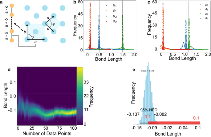
a Schematic illustration of the correspondence between even-odd chains and 2D lattice. b Final posterior distributions of parameters (µ1, µ2, σ1, and σ2) involved in analysis of case-1, posterior distributions after first update are shown by solid lines. c Final posterior distributions of parameters (µ1, µ2, σ1, and σ2) involved in case-2, posterior distributions after first update are shown by solid lines. d Posterior distribution of µ3 as a function of number of datapoints for case-2. e High density interval (HDI) of µ3 (blue) and region of practical importance (ROPE) (red).
For a non-trivial case, odd and even bond lengths are derived from the normal distributions, N(µ = 0.95, σ2 = 0.01) and N(µ = 1.05, σ2 = 0.01). Here, the difference in the means is on the order of the standard deviation. We refer to this analysis as case-2. Figure 1b shows the final posterior distributions of the parameters involved, with the posterior distributions after the first update shown by the solid lines. To answer the question of whether the set of bond lengths belong to a simple chain or a diatomic chain, we construct the distribution of the difference in bond lengths with a likelihood, N(µ = µ3, σ = σ3). For a simple ideal lattice, this distribution should be centered at zero with no standard deviation. Figure 1d shows the posterior distribution for µ3 as a function of the number of datapoints. We then construct an interval region of practical equivalence (ROPE), which is the region around the hypothesis where the hypothesis is still true. A decision on the validity of the hypothesis can be made by comparing the highest density interval (HDI, 94% credible interval) and the ROPE. For illustration purposes, the ROPE is considered to be [−0.1, 0.1] in Fig. 1e and the HDI for µ3 is also shown. Decision rules for different overlaps of HDI and ROPE are discussed in e.g., ref. 70.
This simple example illustrates that for microscopic observations, many fundamental parameters are defined only in the Bayesian sense as the posterior probability densities. They can be related to the macroscopic definitions through concepts such as the practical equivalence. For large system sizes, the Bayesian estimates converge to the macroscopic model. We pose that the Bayesian descriptions of symmetry and structural properties from the bottom up should be Bayesian in nature, updating the prior knowledge of the system with the experimental data.
Local crystallographic analysis
As a second concept, we discuss established approaches for the systematic analysis of atomic structures from experimental observations and the deep fundamental connections between the intrinsic symmetries present (or postulated) in the data and the neural network architectures. For example, the classical fully connected multilayer perceptron intrinsically assumes the presence of potential strong correlations between arbitrarily separated pixels of the input image, resulting in a well-understood limitation of these networks to only relatively low-dimensional features. Convolutional neural networks (CNNs) are introduced as a universal approach for equivariant data analysis where the features of interest can be present anywhere within the image plane. This network architecture implicitly assumes the presence of continuous translational symmetry, similar to the sliding window/transform approach73,74,75. While allowing derivation of mesoscopic information, even for atomically resolved data, this approach suffers from inevitable spatial averaging and ignores the existence of well-defined atomic units.
If the positions of the atomic species can be determined, the analysis can be performed based on the local atomic neighborhoods (local crystallography)76,77 or the full atomic connectivity graph. In these approaches, the full image is reduced to atomic coordinates and the subsequent analysis is based on the latter. It is important to note that in this case all remaining information in the image plane is ignored, i.e., the full data set is approximated by the point estimates of the atomic positions. Finally, the combined approach can be based on the analysis of sub-images centered on defined atomic positions78,79. In this case, the known atomic positions provide the reference points and the sub-images contain information on the structure and functionality around them.
For atomic and sub-image-based descriptors, the behavior referenced to the ideal behavior is of interest and is defined by high-symmetry positions or ideal lattice sites. If these are known, then behaviors such as symmetry-breaking distortions can be immediately quantified and explored. However, the very nature of experimental observations is such that this ground truth information is not available directly, necessitating suitable approximations. For example, an ideal lattice can be postulated and average parameters can be found using a suitable filtering method. However, this approach is sensitive to minute distortions of the image (e.g., due to drift) and image distortion correction is required. Similarly, variability in the observed images due to microscope configurations (mis-tilt, etc.) can provide observational biases.
These examples illustrate that deep analysis of the structure and symmetry from atomically resolved data sets necessitates simultaneous (a) identification of ideal building blocks and symmetry breaking distortions, while (b) allowing for general rotational invariance in the image plane and (c) accounting for discrete translational symmetry as implemented in the Bayesian setting. Ideally, such descriptors will be referenced to local features.
Bayesian local crystallography
Here, we aim to combine the local crystallography and Bayesian approaches. The general workflow for deep Bayesian local crystallographic analysis is shown in Fig. 2a. For the first step, the STEM image or a stack of images are fed into the deep fully convolutional neural network (DCNN). for semantic segmentation and atom finding80,81. The semantics segmentation refers to a process where each pixel in the raw experimental data is categorized as belonging to an atom (or to a particular type of atom) or to a “background” (vacuum). The atom finding procedure is then performed on segmented data by finding a center of the mass of each segmented blob (corresponding to an atom) with a sub-pixel precision. The details of the DCNN configuration and implementation are available via the AtomAI repository on GitHub82. The DCNN-derived atomic positions are used to define the stack of sub-images centered on each atom and represent the image contrast in the vicinity of each atom.
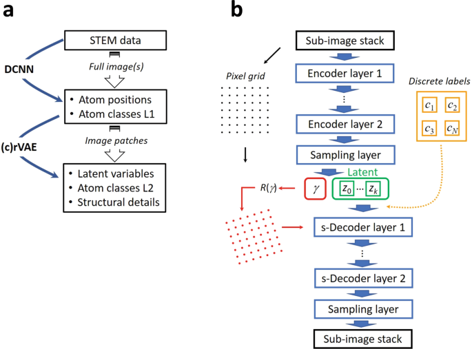
a General workflow of deep Bayesian local crystallographic analysis. b Schematic of (conditional) rotational variational autoencoder, (c)rVAE, workflow. In (c)rVAE, the encoder layers can be either fully connected or convolutional, whereas the decoder layers are always fully-connected layers (in the current implementation, inclusion of convolutional layers breaks the rotational symmetry).
Note that this sub-image description is chosen since both the original STEM data and DCNN reconstructions contain information beyond atomic coordinates, such as column shapes and unresolved features, and this needs to be taken into account during analysis. It is important to note that the choice of sub-image stack (original image, smoothed image, or DCNN output) defines the type of information that will be explored. For example, DCNN outputs define the probability density that a certain image pixel belongs to a given atom class that is optimal for exploration of chemical transformation pathways. At the same time, original image contrast may be optimal for exploration of physical phenomena. Finally, we note that the extremely important issue in this analysis is the correction of distortions for effects such as fly-back delays or general image instabilities, which can alleviate unwanted artifacts and introduce new ones. Several examples of these will be discussed below. If necessary, these sub-images can be used to further refine the classes using standard methods such as principal component analysis (PCA) or Gaussian mixture modelling (GMM). GMM is a type of clustering technique that assumes that each cluster is a multivariate normal distribution. The clusters are characterized by a mean and a covariance matrix. The parameters (means and covariance matrices) of the clusters are estimated by maximum a posteriori estimation83. However, as mentioned above, these clustering methods will tend to separate the atoms into symmetry equivalent positions, leading to over-classification and poorly separable classes.
To avoid this problem, the subsequent step in the analysis is the rotationally invariant variational autoencoder (rVAE). In general, VAE is a directed latent-variable probabilistic graphical model. It allows learning stochastic map** between an observed x-space (in this case, space of the sub-images) with a complicated empirical distribution and a latent z-space whose distribution can be relatively simple84. Recently, it has been used by a subset of authors for exploring the (latent) order parameter from imaging data on dynamically evolving systems ranging from monolayer graphene85 to protein nanoparticles86. More specifically, the VAE consists of generative and inference models, which are Bayesian networks of the form \(p\left( {x|z} \right)p(z)\) and \(q\left( {z|x} \right)\), respectively. For the generative model, the latent variable, zi, is a “code” (hidden representation) from which it reconstructs xi. The potentially complex, non-linear dependency between xi and zi is parameterized by a (deep) neural network (NN) with weights θ, \(p_\theta \left( {x|z} \right)\), which takes “code” zi as an input. The inference model is used to approximate the posterior of the generative model, \(p_\theta \left( {z|x} \right)\), and represents a flexible family of variational distributions parameterized by a NN with weights ϕ, \(q_\phi \left( {z|x} \right)\). The NN-parameterized inference and generative models are frequently referred to as encoder and decoder, respectively. The point estimates for the parameters of the two networks (θ and ϕ) are jointly learned by maximizing the evidence lower boundary (ELBO) consisting of the reconstruction loss term and Kullback-Leibler (KL) divergence term with a mini-batch stochastic gradient descent (SGD). We note that a fully Bayesian treatment of the encoder and decoder weights is also possible, in which case the mini-batch SGD training procedure is substituted by a full-batch Hamiltonian Monte Carlo. However, as of now, aside from extremely high computational costs, the fully Bayesian neural networks show surprisingly poor performance on the data corrupted by noise87, which makes them potentially suboptimal for experimental data.
Here, we aim to learn a rotationally invariant code for our data. Unfortunately, standard neural network layers (fully connected and convolutional) do not respect rotational symmetry or invariance. One potential way to circumvent this problem is to use convolutional layers with modified, steerable filters88. Another approach, which is specific to the VAE set up, is to disentangle rotations from image content by making the generative model (decoder) explicitly dependent on the coordinates (Fig. 2b)89. In this case, we sample our ‘latent angle’ from a prescribed distribution (more details below) and use it to perform a 2D rotation of the coordinate grid, \(R\left( \gamma \right){{{{{\mathbf{x}}}}}}_g\). The rotated grid is then passed to a decoder where it is concatenated with “standard” VAE latent variables. Overall, the generative process is defined as
where \(p\left( z \right)\) is a standard normal prior for the continuous latent code, \(p\left( \gamma \right)\) is a normal prior for the latent angle \(\gamma\) with a “rotational prior” \(s_\gamma ^2\) set by a user, and \(Bern\left( {x|g\left( {z,\gamma } \right)} \right)\) is a parametrized Bernoulli likelihood function where \(g\) is a decoder NN with the coordinate transformation (followed by the concatenation) as an “input layer”. We note that while priors other than Normal, including von Mises and projected normal distributions90, can in principle be used for the latent angle, we did not find empirically any significant difference in the results for the dataset discussed in this paper. The encoder in our inference model outputs the approximate parameters of the posterior distribution,
where \(\mu _\phi \left( x \right)\) and \({\upsigma}_\phi ^2\left( x \right)\) correspond to the multi-head encoder NN. The loss objective (the negative ELBO) is computed as
where the first term is a reconstruction error (which, in case of Bernoulli likelihood, is equivalent to a binary cross-entropy loss), and the second and third terms are the KL divergences associated with image content and rotation angle, respectively.
Hence, for the rVAE, the latent space is configured to comprise the rotational angle and additional unstructured latent variables. We note that other (than rotation) affine transformations including lateral offsets and scale can be added as well. These VAE configurations are ideally suited for the analysis of the variability in the STEM sub-image stack since uncertainties in the atomic positions (if any) can be naturally accommodated through the offset latent variables and the continuous or discrete rotations are captured by the angle variable. The remaining latent variables can be used in a manner similar to classical variational autoencoders4. The latent space distribution exhibits extremely interesting behavior. Figure 5a shows the joint distribution of the latent variables, visualized both as individual points and with a superimposed kernel density estimate (KDE). Note that each point corresponds to the sub-image and describes the behavior of the local neighborhood of a single lattice atom. The representation as points and KDE allows the comparison between the total system behavior (including the distribution of outliers) and the corresponding densities (average behaviors) and is necessary given the large number of points (from ~104 for single images to ~105 for the stacks).
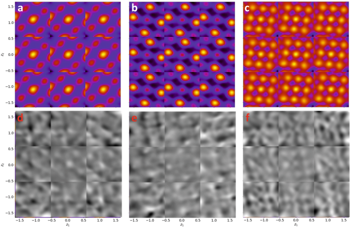
Conditional rVAE analysis of the three GMM components from Fig. 4 corresponding to the a, d A-site (component 1), b, e B-site (component 2) columns of the LSMO phase and c, f NiO phase (component 3). The upper images are the raw images, and the lower images have the average of the 3×3 tableau subtracted.
To extend this analysis, we note that the rVAE often tends to disentangle dissimilar types of distortions within a system. For example, experiments with a large number of different STEM images (beyond those shown in this paper) illustrate that scan distortions often tend to be described by one (group of) latent variables, whereas systematic changes in the local structure are described by the remaining latent variables. This property of VAEs is generally well known in computer science applications such as style networks; however, here we see that it applies for the physical systems as well.
We further explore this separation of atomic units based on neighborhood behavior using disentangled representations. As observed in Fig. 3, the angle and latent variable 2 seem to offer the optimal 2D basis to separate the atomic units, with clear contrast and a lack of distortion behaviors. The corresponding distribution and KDE plots are shown in Fig. 4b, illustrating three clearly defined groups of points corresponding to the A-site and B-site cations in the LSMO phase and columns in the NiO phases, respectively. Note that the KDE peaks corresponding to the three atomic types that jointly comprise >90% of points are fairly narrow. At the same time, there are a large number of outliers showing the presence of atoms with the behaviors falling on the continuous lines between the three groups, forming the manifold of possible states in the system.
Finally, we can gain further insight into the spatial distributions and classes of behaviors via clustering in the latent space. Figure 4c shows the Gaussian mixture model (GMM) clustering of points in the latent space. Note that given the complex structure of the distribution, the choice of a proper covariance matrix for the GMM, or the exploration of different clustering methods, will highlight different aspects of system behavior and hence offer a powerful tool for the exploration of corresponding physics. Here, we show as an example of the separation in three components. The spatial distribution of the label maps is shown in Fig. 4b and images corresponding to the centroids of the GMM classes are shown in Fig. 4e–g. Components 1 (blue) and 2 (green) correspond to the A and B sites in the perovskite, respectively, while component 3 (brown) corresponds to the NiO phase. To examine if additional components can provide more information, we repeat the analysis for five components in Fig. S5. The GMM analysis, shown in Fig. S5a, shows four well-defined clusters with one component more widely distributed. The spatial distribution of the components is shown in Fig. S5b while the individual components are shown in Fig. S5c–g. Once again, the first two components correspond to the A and B sites of the perovskite and fourth component corresponds to the NiO phase. The third component, which is the distributed component in the GMM cluster plot. It corresponds to a distorted NiO lattice and occurs at the edges of the NiO inclusions at the interface with the LSMO phase. The fifth component corresponds to a distorted A site in the LSMO. This is distributed throughout the perovskite lattice, with some horizontal stripes corresponding to the previously discussed scan distortions. The analysis is repeated on the DCNN segmented image shown in Fig. S6. In this case components 1 and 3 correspond to the LSMO lattice and component 2 corresponds to the NiO phase. Components 1 and 3 are no longer easily identified as the A or B sites of the perovskite but appear to be related by rotation. The distribution of these components is essentially random throughout the LSMO lattice rather than showing an alternating pattern seen in Fig. 4b. This most like due to the loss of intensity and shape information due to semantic segmentation.
To get further insight into the materials structure, we explore the disentangled representations of the structural building blocks using the conditional rotationally invariant variational autoencoder (crVAE) approach. The schematics of crVAE is shown in Fig. 2. Here, the autoencoder approach is used on the concatenated image stack (or its reduced representation) and the class labels. At the decoding stage, the mini-batch with one-hot encoded labels is concatenated with the unstructured latent variables. This leads to the decoder probability distribution being conditioned on the continuous latent code z and discrete labels c, \(p_\theta \left( {z|x,c} \right)\). The typical example of the crVAE application will be disentanglement of the styles in the MNIST data set93. Whence simple VAE will draw all the numbers and distribute them in the latent space, the crVAE will draw the selected number and the latent space representations will reflect writing styles—e.g. tilt, line width, etc. The key aspect of using crVAE approach, as opposed of VAE analysis of individual classes, is that the thus disentangled styles will be common across the data set, reminiscent of hierarchical Bayesian models. If the labels are known only partially, the unknown discrete classes are sampled from a uniform categorical distribution and an additional classifier neural network is added turning the model into a semi-supervised generative model. Recently, a subset of authors has shown that a semi-supervised rVAE model can be used for creating nanoparticle libraries from imaging data94. Here, we will limit ourselves to a scenario where all labels are known.
As an example of crVAE analysis, shown in Fig. 5 is the latent space representation for the three GMM components of the LSMO–NiO system form Fig. 4. Here, the latent space is subdivided into 3 × 3 regions and the corresponding images are reconstructed. Shown are the images per se and the images with subtracted average. Note that while direct physical interpretation of this disentangled representations is complex, we note the commonality in the character of changes in the vertical and lateral directions for all three components. The central position of each tableau shows the least variation from the mean value, with higher than average values seen to the left and lower than average values to the right.
Application of rVAE to a layered perovskite
We can extend this analysis to a system with a significantly more complex lattice such as the Sr3Fe2O7 (SFO) layered perovskite. Sr3Fe2O7 is a mixed valence Ruddlesden-Popper series compound with double perovskite structure that nominally features tetravalent iron. Charge disproportionation to Fe(III) and Fe(V) was observed by Mössbauer spectroscopy95,96. Spiral magnetic order was observed by neutron diffraction97 and provides a rare example of a magnetic cycloid arising from a ferromagnetic nearest neighbor competing with antiferromagnetic next-nearest exchange98. Further interest in this material arise from high oxygen mobility99. The preparation of a near stoichiometric compound requires high oxygen partial pressure100.
The rVAE analysis of SFO is shown in Fig. 6. The original STEM image, Fig. 6a, clearly illustrates the layered structure of SFO. In Fig. 6b the sub-image representation of the of the latent variable shows a change of contrast from left to right and a change of structure towards the top. Of most interest is the encoded angle, Fig. 6c, which shows three separate values, one down the center of the layers and alternating values either side. The histogram of the encoded angle is shown in Fig. 6f where three peaks are clearly present. The peaks have been labeled with colored circles corresponding to those on Fig. 6c. The first latent space in Fig. 6d exhibits a more complex periodic structure consistent with the corresponding four peaked histogram shown in Fig. 6g. The second latent space exhibits a gradual change in intensity from left to right corresponding to the sample thickness variation, which is also observed in the raw STEM image (Fig. 6a). The corresponding histogram has a flattened peak corresponding to this gradual change. Similar to observations for a 2-phase system, these behaviors are now disentangled and can be explored separately. We observed a similar separation for other STEM images where scan distortions e.g., due to fly-back delays, were clearly concentrated in a single latent variable.
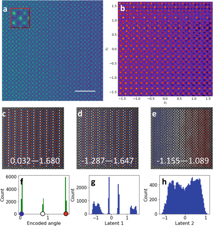
a Original STEM image with a sub-image inlayed in the red box. The scale bar is 2 nm b sub-image representation in 2D latent parameter space, c encoded angle, d latent Z1 e latent variable Z2. and f–h, the histograms corresponding to c–e. The circles on f correspond to the points on c. Analysis is performed on raw images using window size of 40 pixels. Insets indicate intensity variation of each panel.
The choice of window size is crucial for extracting some of these features. The effect of using a smaller and larger window size on the rVAE process is shown in Fig. S7. The 2D latent parameter space for 32 pixels, shown in Fig S7a shows a gradual change in contrast from left to right. The encoded angle in Fig. S7c is basically constant in value. Examination of the associated histogram (Fig. S7f) shows that the three peaks seen in Fig. 6f have collapsed to a single sharp peak. The latent variables show a gradual change in in tensity from left to right similar to that seen in Fig. 6e. The results are similar for a larger window size of 60 pixels. It should be noted that the intermediate values the encoded angle histograms first lose the central peak before collapsing to a single peak. For completeness, this analysis was also performed on the DCNN segmented images and the results are shown in Fig. S8 and S9. To obtain the same three peaked encoded angle histogram a window of 34 pixels was used. The peaks on either extreme are separated by a full 180 degrees and are represented by the red and blue markers on Fig. S8c. They represent the atoms at the edge of the bands. The range for the raw image analysis was approximately half of this, perhaps because of the noise level of the original data. The first latent variable still reflects the banded structure but the second is basically random. The results for the DCNN segmented data are extremely sensitive to window size. As seen in Fig S9, varying the window size by 2 pixels either way the three peaked encoded angle histogram is reduce to either one or two peaks.
For completeness a clustering analysis has been performed on the SFO results and these results and discussion are included in the supplementary information (Figs. S10 and S11).
To summarize, we introduce a workflow for the bottom-up symmetry and structural analysis of atomically resolved STEM imaging data. For systems with known or ad hoc defined rotational variants, the combination of Gaussian mixture modeling and principal component analysis (GMM-PCA) allows separation of the relevant structural units and structural distortions for individual units. However, the GMM-PCA combination fails in the presence of multiple rotational variants and especially general rotations, since in this case the class will be assigned to each rotation of the same structural unit. The use of the rVAE-crVAE approach proposed here allows one to generalize the classification-distortion analysis for the general rotational symmetry. We illustrate that the capability of VAEs to produce disentangled representations can be beneficially used to separate structural units, relevant distortions, and in certain cases, the instrumental distortions, opening the pathway for systematic studies of symmetry breaking distortions for a broad range of material systems.
While implemented here for the analysis of structural STEM images, we expect that a similar approach can be used for the analysis of symmetry breaking distortions in e.g., scanning tunneling microscopy (STM) images, and can be further extended to the analysis of multidimensional data sets such as tunneling spectroscopy in STM, EELS and 4D STEM in STEM, and so on. Furthermore, similar to other Bayesian methods, it will be of interest to explore physics-based prior distributions in the latent space, beyond the class labels used here. Overall, we believe that the combination of the capability to disentangle physical phenomena via latent space representations and parsimonious analysis makes the proposed workflow universal for multiple physical problems.
Methods
Thin film growth
The LSMO–NiO VAN and the single-phase LSMO and NiO films were grown on STO(001) single-crystal substrates by PLD using a KrF excimer laser (λ = 248 nm) with fluence of 2 J/cm2 and a repetition rate of 5 Hz. All films were grown at 200 mTorr O2 and 700 °C. The films were post-annealed in 200 Torr of O2 at 700 °C to ensure full oxidation, and cooled down to room temperature at a cooling rate of 20 °C/min. For out-of-plane transport measurements, the films were grown on 0.5% Nb-doped STO(001) single-crystal substrates. The film composition was varied by using composite laser ablation targets with different composition.
Sample preparation
A polycrystalline rod of Sr3Fe2O7-x with 6 mm in diameter and 50 mm in length was prepared using powders synthesized from solid state reaction of stoichiometric SrCO3 and Fe2O3 at 1100 °C. The single crystalline material utilized here was grown using a high pressure floating zone furnace with O2 partial pressure of 148 bar. Refinement of neutron diffraction data obtained at the NOMAD instrument of the Spallation Neutron Source using GSAS-II101 revealed a single-phase material with an oxygen content of 6.8, see Supplementary Fig. S12 and Table S1.
STEM
The plan-view STEM samples of Ni-LSOM were prepared using ion milling after mechanical thinning and precision polishing. In brief, a thin film sample was firstly ground, and then dimpled and polished to a thickness less than 20 micrometer from the substrate side. The sample was then transferred to an ion milling chamber for further substrate-side thinning. The ion beam energy and milling angle were adjusted towards lower values during the thinning process, which was stopped when an open hole appeared for STEM characterization. The Sr3Fe2O7 sample(s) were prepared by FIB lift out followed by local low energy Ar ion milling, down to 0.5 eV, in a Fischione NanoMill.
The STEM used for the characterization of both samples was a Nion UltraSTEM200 operated at 200 kV. The beam illumination half-angle was 30 mrad and the inner detector half-angle was 65 mrad. Electron energy-loss spectra were obtained with a collection half-angle of 48 mrad.
Data availability
The Jupyter notebook containing links to the data and used for this analysis is available at https://github.com/markpoxley/Bayesian_Crystallography.
References
Smith, C. S. in Solid State Physics Vol. 6 (eds Frederick Seitz & David Turnbull) 175–249 (Academic Press, 1958).
Kittel, C. Introduction to Solid State Physics. (Wiley, 2004).
Ashcroft, N. W. & Mermin, N. D. Solid State Physics (Holt, Rinehart and Winston, 1976).
Malgrange, C., Ricolleau, C. & Schlenker, M. Symmetry and Physical Properties of Crystals. (Springer Netherlands, 2014).
Birss, R. R. Macroscopic symmetry in space-time. Rep. Prog. Phys. 26, 307–360 (1963).
Powell, R. C. Symmetry, Group Theory, and the Physical Properties of Crystals (Springer New York, 2010).
Marder, M. P. Condensed Matter Physics. (Wiley, 2010).
Bursill, L. A. & Ju Lin, P. Penrose tiling observed in a quasi-crystal. Nature 316, 50–51 (1985).
Kumar, V., Sahoo, D. & Athithan, G. Characterization and decoration of the two-dimensional Penrose lattice. Phys. Rev. B 34, 6924–6932 (1986).
Steinhardt, P. J. & Jeong, H.-C. A simpler approach to Penrose tiling with implications for quasicrystal formation. Nature 382, 431–433 (1996).
Tang, L.-H. & Jarić, M. V. Equilibrium quasicrystal phase of a Penrose tiling model. Phys. Rev. B 41, 4524–4546 (1990).
Levine, D. & Steinhardt, P. J. Quasicrystals: a new class of ordered structures. Phys. Rev. Lett. 53, 2477–2480 (1984).
Steinhardt, P. J. & Ostlund, S. The Physics of Quasicrystals (World Scientific, 1987).
Glinchuk, M. D. & Stephanovich, V. A. Dynamic properties of relaxor ferroelectrics. J. Appl. Phys. 85, 1722–1726 (1999).
Vugmeister, B. E. Polarization dynamics and formation of polar nanoregions in relaxor ferroelectrics. Phys. Rev. B 73, 174117 (2006).
Takenaka, H., Grinberg, I., Liu, S. & Rappe, A. M. Slush-like polar structures in single-crystal relaxors. Nature 546, 391–395 (2017).
Binder, K. & Reger, J. D. Theory of orientational glasses models, concepts, simulations. Adv. Phys. 41, 547–627 (1992).
Binder, K. & Young, A. P. Spin-glasses—experimental facts, theoretical concepts, and open questions. Rev. Mod. Phys. 58, 801–976 (1986).
Dagotto, E. Complexity in strongly correlated electronic systems. Science 309, 257–262 (2005).
Dagotto, E., Hotta, T. & Moreo, A. Colossal magnetoresistant materials: The key role of phase separation. Phys. Rep. Rev. Sec. Phys. Lett. 344, 1–153 (2001).
Blinc, R. et al. Local polarization distribution and Edwards-Anderson order parameter of relaxor ferroelectrics. Phys. Rev. Lett. 83, 424–427 (1999).
Cross, L. E. Relaxor ferroelectrics. Ferroelectrics 76, 241–267 (1987).
Cliffe, M. J. et al. Structural simplicity as a restraint on the structure of amorphous silicon. Phys. Re. B 95, 224108 (2017).
Keen, D. A. & Goodwin, A. L. The crystallography of correlated disorder. Nature 521, 303–309 (2015).
Cheetham, A. K., Bennett, T. D., Coudert, F. X. & Goodwin, A. L. Defects and disorder in metal organic frameworks. Dalton Trans. 45, 4113–4126 (2016).
Gerber, C. & Lang, H. P. How the doors to the nanoworld were opened. Nat. Nanotechnol. 1, 3–5 (2006).
Binnig, G., Rohrer, H., Gerber, C. & Weibel, E. 7x7 Reconstruction on si(111) resolved in real space. Phys. Rev. Lett. 50, 120–123 (1983).
Binnig, G., Quate, C. F. & Gerber, C. Atomic force microscope. Phys. Rev. Lett. 56, 930–933 (1986).
Dellby, N., Krivanek, O. L., Nellist, P. D., Batson, P. E. & Lupini, A. R. Progress in aberration-corrected scanning transmission electron microscopy. J. Electron Microsc. 50, 177–185 (2001).
Batson, P. E., Dellby, N. & Krivanek, O. L. Sub-angstrom resolution using aberration corrected electron optics. Nature 418, 617–620 (2002).
Krivanek, O. L. et al. Atom-by-atom structural and chemical analysis by annular dark-field electron microscopy. Nature 464, 571–574 (2010).
Krivanek, O. L., Dellby, N., Spence, A. J., Camps, R. A. & Brown, L. M. in Electron Microscopy and Analysis 1997 Institute of Physics Conference Series (ed J. M. Rodenburg) 35–40 (Iop Publishing Ltd, 1997).
Yankovich, A. B. et al. Picometre-precision analysis of scanning transmission electron microscopy images of platinum nanocatalysts. Nat. Commun. 5, 4155 (2014).
Ray, N. & Waghmare, U. V. Coupling between magnetic ordering and structural instabilities in perovskite biferroics: A first-principles study. Phys. Rev. B 77, 10 (2008).
Zhou, J. S. & Goodenough, J. B. Universal octahedral-site distortion in orthorhombic perovskite oxides. Phys. Rev. Lett. 94, 4 (2005).
Radaelli, P. G. & Cheong, S. W. Structural phenomena associated with the spin-state transition in LaCoO(3). Phys. Rev. B 66, 9 (2002).
Kanamori, J. Crystal distortion in magnetic compounds. J. Appl. Phys. 31, S14–S23 (1960).
Imada, M., Fujimori, A. & Tokura, Y. Metal-insulator transitions. Rev. Mod. Phys. 70, 1039–1263 (1998).
Tokura, Y. & Nagaosa, N. Orbital physics in transition-metal oxides. Science 288, 462–468 (2000).
Goodenough, J. B. An interpretation of the magnetic properties of the perovskite-type mixed crystals la1-xsrxcoo3-lambda. J. Phys. Chem. Solids 6, 287–297 (1958).
Jia, C. L. et al. Unit-cell scale map** of ferroelectricity and tetragonality in epitaxial ultrathin ferroelectric films. Nat. Mater. 6, 64–69 (2007).
Pan, X. Q., Kaplan, W. D., Ruhle, M. & Newnham, R. E. Quantitative comparison of transmission electron microscopy techniques for the study of localized ordering on a nanoscale. J. Am. Ceram. Soc. 81, 597–605 (1998).
Nelson, C. T. et al. Spontaneous Vortex Nanodomain Arrays at Ferroelectric Heterointerfaces. Nano Lett. 11, 828–834 (2011).
Chisholm, M. F., Luo, W. D., Oxley, M. P., Pantelides, S. T. & Lee, H. N. Atomic-scale compensation phenomena at polar interfaces. Phys. Rev. Lett. 105, 197602 (2010).
Kim, Y. M. et al. Direct observation of ferroelectric field effect and vacancy-controlled screening at the BiFeO3/LaxSr1-xMnO3 interface. Nat. Mater. 13, 1019–1025 (2014).
Borisevich, A. Y. et al. Suppression of octahedral tilts and associated changes in electronic properties at epitaxial oxide heterostructure interfaces. Phys. Rev. Lett. 105, 087204 (2010).
Jia, C. L. et al. Oxygen octahedron reconstruction in the SrTiO(3)/LaAlO(3) heterointerfaces investigated using aberration-corrected ultrahigh-resolution transmission electron microscopy. Phys. Rev. B 79, 081405 (2009).
He, Q. et al. Towards 3D map** of BO6 octahedron rotations at perovskite heterointerfaces, unit cell by unit cell. ACS Nano 9, 8412–8419 (2015).
Ozdol, V. B. et al. Strain map** at nanometer resolution using advanced nano-beam electron diffraction. Appl. Phys. Lett. 106, 253107 (2015).
Feist, A., Silva, N. R. D., Liang, W., Ropers, C. & Schäfer, S. Nanoscale diffractive probing of strain dynamics in ultrafast transmission electron microscopy. Struct. Dyn. 5, 014302 (2018).
Yuan, R., Zhang, J., He, L. & Zuo, J.-M. Training artificial neural networks for precision orientation and strain map** using 4D electron diffraction datasets. Ultramicroscopy, 113256, https://doi.org/10.1016/j.ultramic.2021.113256 (2021).
Borisevich, A. Y. et al. Exploring Mesoscopic Physics of Vacancy-Ordered Systems through Atomic Scale Observations of Topological Defects. Phys. Rev. Lett. 109, 065702 (2012).
Li, Q. et al. Quantification of flexoelectricity in PbTiO3/SrTiO3 superlattice polar vortices using machine learning and phase-field modeling. Nat. Commun. 8, 1468 (2017).
Vlcek, L. et al. Learning from imperfections: predicting structure and thermodynamics from atomic imaging of fluctuations. ACS Nano 13, 718–727 (2019).
Vlcek, L., Maksov, A., Pan, M. H., Vasudevan, R. K. & Kahnin, S. V. Knowledge extraction from atomically resolved images. ACS Nano 11, 10313–10320 (2017).
Vlcek, L., Vasudevan, R. K., Jesse, S. & Kalinin, S. V. Consistent integration of experimental and ab initio data into effective physical models. J. Chem. Theory Comput. 13, 5179–5194 (2017).
Hytch, M. J. & Potez, L. Geometric phase analysis of high-resolution electron microscopy images of antiphase domains: example Cu3Au. Philos. Mag. A 76, 1119–1138 (1997).
Kioseoglou, J., Dimitrakopulos, G. P., Komninou, P., Karakostas, T. & Aifantis, E. C. Dislocation core investigation by geometric phase analysis and the dislocation density tensor. J. Phys. D.Appl. Phys. 41, 8 (2008).
Peters, J. J. P. et al. Artefacts in geometric phase analysis of compound materials. Ultramicroscopy 157, 91–97 (2015).
Zhao, C. W., **ng, Y. M., Zhou, C. E. & Bai, P. C. Experimental examination of displacement and strain fields in an edge dislocation core. Acta Mater. 56, 2570–2575 (2008).
Hytch, M. J., Putaux, J. L. & Thibault, J. Stress and strain around grain-boundary dislocations measured by high-resolution electron microscopy. Philos. Mag. 86, 4641–4656 (2006).
Feenstra, R. M. & Stroscio, J. A. Tunneling spectroscopy of the gaas(110) surface. J. Vac. Sci. Technol. B 5, 923–929 (1987).
Sugimoto, Y. et al. Chemical identification of individual surface atoms by atomic force microscopy. Nature 446, 64–67 (2007).
Dobigeon, N. & Brun, N. Spectral mixture analysis of EELS spectrum-images. Ultramicroscopy 120, 25–34 (2012).
Pennycook, S. J., Varela, M., Lupini, A. R., Oxley, M. P. & Chisholm, M. F. Atomic-resolution spectroscopic imaging: past, present and future. J. Electron Microsc. 58, 87–97 (2009).
Jesse, S. et al. Big data analytics for scanning transmission electron microscopy ptychography. Sci. Rep. 6, 26348 (2016).
Jiang, Y. et al. Electron ptychography of 2D materials to deep sub-angstrom resolution. Nature 559, 343–349 (2018).
Nellist, P. D., McCallum, B. C. & Rodenburg, J. M. Resolution beyond the information limit in transmission electron-microscopy. Nature 374, 630–632 (1995).
Kruschke, J. Doing Bayesian Data Analysis: A Tutorial with R, JAGS, and Stan, 2nd edn. (Academic Press, 2014).
Martin, O. Bayesian Analysis with Python: Introduction to statistical modeling and probabilistic programming using PyMC3 and ArviZ, 2nd Edn. (Packt Publishing, 2018).
Lambert, B. A Student’s Guide to Bayesian Statistics, 1st edn. (SAGE Publications Ltd, 2018).
Ghahramani, Z. Probabilistic machine learning and artificial intelligence. Nature 521, 452–459 (2015).
Vasudevan, R. K., Ziatdinov, M., Jesse, S. & Kalinin, S. V. Phases and interfaces from real space atomically resolved data: physics-based deep data image analysis. Nano Lett. 16, 5574–5581 (2016).
Vasudevan, R. K. et al. Big data in reciprocal space: Sliding fast Fourier transforms for determining periodicity. Appl. Phys. Lett. 106, 091601 (2015).
He, Q., Woo, J., Belianinov, A., Guliants, V. V. & Borisevich, A. Y. Better catalysts through microscopy: mesoscale M1/M2 intergrowth in molybdenum-vanadium based complex oxide catalysts for propane ammoxidation. ACS Nano 9, 3470–3478 (2015).
Lin, W. Z. et al. Local crystallography analysis for atomically resolved scanning tunneling microscopy images. Nanotechnology 24, 415707 (2013).
Belianinov, A. et al. Identification of phases, symmetries and defects through local crystallography. Nat. Commun. 6, 7801 (2015).
Ziatdinov, M., Nelson, C., Vasudevan, R. K., Chen, D. Y. & Kalinin, S. V. Building ferroelectric from the bottom up: the machine learning analysis of the atomic-scale ferroelectric distortions. Appl. Phys. Lett. 115, 5 (2019).
Ziatdinov, M., Dyck, O., Jesse, S. & Kalinin, S. V. Atomic mechanisms for the Si atom dynamics in graphene: chemical Transformations at the edge and in the bulk. Adv. Funct. Mater. 29, 8 (2019).
Ziatdinov, M. et al. Building and exploring libraries of atomic defects in graphene: scanning transmission electron and scanning tunneling microscopy study. Sci. Adv. 5, eaaw8989 (2019).
Ziatdinov, M. et al. Deep learning of atomically resolved scanning transmission electron microscopy images: chemical identification and tracking local transformations. ACS Nano 11, 12742–12752 (2017).
Ziatdinov, M. AtomAI. GitHub repository, https://github.com/pycroscopy/atomai (2020).
Mohammed, M., Khan, M. B. & Bashier, E. B. M. Machine Learning: Algorithms and Applications. (CRC Press, 2016).
Kingma, D. P. & Welling, M. Auto-encoding variational bayes. ar**v:1312.6114. Preprint at https://arxiv.org/abs/1312.6114 (2013).
Kalinin, S. V., Dyck, O., Jesse, S. & Ziatdinov, M. Exploring order parameters and dynamic processes in disordered systems via variational autoencoders. Sci. Adv. 7, eabd5084 (2021).
Kalinin, S. V. et al. Disentangling rotational dynamics and ordering transitions in a system of self-organizing protein nanorods via rotationally invariant latent representations. ACS Nano 15, 6471–6480 (2021).
Izmailov, P., Vikram, S., Hoffman, M. D. & Wilson, A. G. What are Bayesian neural network posteriors really like? ar**v:2104.14421. Preprint at https://arxiv.org/abs/2104.14421 (2021).
Weiler, M., Hamprecht, F. A. & Storath, M. Learning steerable filters for rotation equivariant CNNs. Proceedings of the IEEE Conference on Computer Vision and Pattern Recognition, 849–858 (2018).
Bepler, T., Zhong, E., Kelley, K., Brignole, E. & Berger, B. Explicitly disentangling image content from translation and rotation with spatial-VAE. Advances in Neural Information Processing Systems, 15409–15419 (2019).
Daniel, H.-S., Breidt, F. J. & Mark, JvdW. The general projected normal distribution of arbitrary dimension: modeling and bayesian inference. Bayesian Anal. 12, 113–133 (2017).
Kingma, D. P. & Ba, J. Adam: A Method for Stochastic Optimization. ar**v:1412.6980. Preprint at https://arxiv.org/abs/1412.6980 (2015).
Paszke, A. et al. Pytorch: an imperative style, high-performance deep learning library. Adv. Neural Inf. Process. Syst. 32, 8026–8037 (2019).
Sohn, K., Lee, H. & Yan, X. Learning structured output representation using deep conditional generative models. Adv. Neural Inf. Process. Syst. 28, 3483–3491 (2015).
Ziatdinov, M., Yaman, M. Y., Liu, Y., Ginger, D. & Kalinin, S. V. Semi-supervised learning of images with strong rotational disorder: assembling nanoparticle libraries. ar**v:2105.11475. Preprint at https://arxiv.org/abs/2105.11475 (2021).
Dann, S. E., Weller, M. T., Currie, D. B., Thomas, M. F. & Al-Rawwas, A. D. Structure and magnetic properties of Sr2FeO4 and Sr3Fe2O7 studied by powder neutron diffraction and Mössbauer spectroscopy. J. Mater. Chem. 3, 1231–1237 (1993).
Kuzushita, K., Morimoto, S., Nasu, S. & Nakamura, S. Charge disproportionation and antiferromagnetic order of Sr3Fe2O7. J. Phys. Soc. Jpn. 69, 2767–2770 (2000).
Kim, J.-H. et al. Competing exchange interactions on the verge of a metal-insulator transition in the two-dimensional spiral magnet Sr3Fe2O7. Phys. Rev. Lett. 113, 147206 (2014).
Fishman, R. S., Rõõm, T. & De Sousa, R. Normal modes of a spin cycloid or helix. Phys. Rev. B 99, 064414 (2019).
Ota, T., Kizaki, H. & Morikawa, Y. Mechanistic analysis of oxygen vacancy formation and ionic transport in Sr3Fe2O7-δ. J. Phys. Chem. C. 122, 4172–4181 (2018).
Peets, D. et al. Magnetic phase diagram of Sr3Fe2O7-δ. Phys. Rev. B 87, 214410 (2013).
Toby, B. H. & Von Dreele, R. B. GSAS-II: the genesis of a modern open-source all purpose crystallography software package. J. Appl. Crystallogr. 46, 544–549 (2013).
Acknowledgements
This effort (ML, STEM, film growth, sample growth) is based upon work supported by the U.S. Department of Energy (DOE), Office of Science, Basic Energy Sciences (BES), Materials Sciences and Engineering Division (S.V.K., S.V., G.E., W.Z., J.Z., H.Z., and R.P.H.) and was performed and partially supported (R.K.V. and M.Z.) at the Oak Ridge National Laboratory’s Center for Nanophase Materials Sciences (CNMS), a U.S. Department of Energy, Office of Science User Facility. Dr. Matthew Chisholm is gratefully acknowledged for the STEM data used in this work. Dr. Katharine Page is gratefully acknowledged for help in the data acquisition at NOMAD. A portion of this research used resources at the Spallation Neutron Source, a DOE Office of Science User Facility operated by the Oak Ridge National Laboratory. The authors are deeply grateful to Dr. Karren More for careful reading and correcting the manuscript.
Author information
Authors and Affiliations
Contributions
S.V.K. proposed the concept, wrote the initial workflow and first paper draft. M.P.O. investigated effect of window size, produced most figures, and wrote descriptions of results. M.V. performed the 1D chain analysis. R.P.H. initiated sample growth and electron microscopy, helped in neutron diffraction analysis, contributed write-up about Sr3Fe2O7. G.E. coordinated and participated in the fabrication on NiO-LSMO vertically oriented nanostructures and the analysis of data. R.K.V. participated in formulating of the idea and ongoing discussions and data analytics. M.Z. wrote the source code used for the analysis. Wrote the part on (r)VAE. J.Z., H.Z., and W.Z. made samples and performed characterization.
Corresponding author
Ethics declarations
Competing interests
The authors declare no competing interests. Author S.K is a member of the Editorial Board for npj Computational Materials. Author S.K was not involved in the journal’s review of or decisions related to this manuscript.
Additional information
Publisher’s note Springer Nature remains neutral with regard to jurisdictional claims in published maps and institutional affiliations.
Supplementary information
Rights and permissions
Open Access This article is licensed under a Creative Commons Attribution 4.0 International License, which permits use, sharing, adaptation, distribution and reproduction in any medium or format, as long as you give appropriate credit to the original author(s) and the source, provide a link to the Creative Commons license, and indicate if changes were made. The images or other third party material in this article are included in the article’s Creative Commons license, unless indicated otherwise in a credit line to the material. If material is not included in the article’s Creative Commons license and your intended use is not permitted by statutory regulation or exceeds the permitted use, you will need to obtain permission directly from the copyright holder. To view a copy of this license, visit http://creativecommons.org/licenses/by/4.0/.
About this article

Cite this article
Kalinin, S.V., Oxley, M.P., Valleti, M. et al. Deep Bayesian local crystallography. npj Comput Mater 7, 181 (2021). https://doi.org/10.1038/s41524-021-00621-6
Received:
Accepted:
Published:
DOI: https://doi.org/10.1038/s41524-021-00621-6
- Springer Nature Limited
This article is cited by
-
Automatic identification of crystal structures and interfaces via artificial-intelligence-based electron microscopy
npj Computational Materials (2023)
-
Machine learning for automated experimentation in scanning transmission electron microscopy
npj Computational Materials (2023)
-
Versatile domain map** of scanning electron nanobeam diffraction datasets utilising variational autoencoders
npj Computational Materials (2023)